It is clear that if we are interested in the probability that
the first count occurs in the  -th time interval
of amplitude
-th time interval
of amplitude  , we recover `in principle'
a geometric distribution. But since can be
arbitrary small, it makes no sense in numbering the intervals.
Nevertheless, thinking in terms of the
, we recover `in principle'
a geometric distribution. But since can be
arbitrary small, it makes no sense in numbering the intervals.
Nevertheless, thinking in terms of the  Bernoulli
process can be again very useful. Indeed, the probability
that the first count occurs after the
Bernoulli
process can be again very useful. Indeed, the probability
that the first count occurs after the  trial is
equal to the probability that it never occurred in the
trials from 1 to
trial is
equal to the probability that it never occurred in the
trials from 1 to  :
:
In the domain of time, indicating now by  the
time at which the first event can occur,
the probability that this variable is larger than the value
the
time at which the first event can occur,
the probability that this variable is larger than the value  ,
the latter being times ,
is given by
,
the latter being times ,
is given by
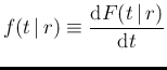
As a complement, the cumulative distribution of , from which
the probability density function follows, is given by
The time at which the first count
is recorded is then described by an exponential
distribution
having expected value, standard deviation and variation coefficient equal to
while the mode (`most probable value')
is always at  , independently
of
, independently
of  .
.
As we can see, as it is reasonable to be,
the higher is the intensity of the process, the
smaller is the expected time at which the first count occurs
(but note that the distribution extends always rather slowly to
 , a mathematical property reflecting the fact that
such a distribution has always a 100% standard uncertainty,
that is
, a mathematical property reflecting the fact that
such a distribution has always a 100% standard uncertainty,
that is  ).
Moreover, since the choice of the instant at which
we start waiting from the first event is arbitrary
(this is related to the so called `property of no memory' of
the exponential distribution, which has an equivalent in the geometric one),
we can choose it
to be the instant at which a previous count occurred.
Therefore, the same distribution describes the time intervals
between the occurrence of subsequent counts.
).
Moreover, since the choice of the instant at which
we start waiting from the first event is arbitrary
(this is related to the so called `property of no memory' of
the exponential distribution, which has an equivalent in the geometric one),
we can choose it
to be the instant at which a previous count occurred.
Therefore, the same distribution describes the time intervals
between the occurrence of subsequent counts.
Once we have got the probability distribution of  , using
probability rules we can get that of
, using
probability rules we can get that of  , reasoning
on the fact that the associated variable is the sum
of two exponentials, and so on. We shall not enter
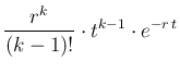
into details,39but only say that we end with the
Erlang distribution, given by
, reasoning
on the fact that the associated variable is the sum
of two exponentials, and so on. We shall not enter
into details,39but only say that we end with the
Erlang distribution, given by
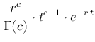
The extension of  to the continuum, indicated for clarity
as
to the continuum, indicated for clarity
as  , leads to the famous
Gamma distribution (here written for our variable )
, leads to the famous
Gamma distribution (here written for our variable )
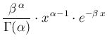
with the `rate parameter' (and it is now clear the reason
for the name) and the `shape parameter'
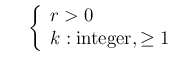
(the special cases in which is integer help to understand its meaning),
having expected value and standard deviation equal to
 and
and
 , both having the dimensions of time
(this observation helps to remember their expression).
, both having the dimensions of time
(this observation helps to remember their expression).
However, since in the text the symbol is assigned to the
intensity of the physical process of interest, we
are going to use for the Gamma distribution the standard symbols
met in the literature (see e.g. [31]
and [32]) applying the following
replacements:
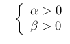
Using also the usual symbol  for generic variable, here is
a summary of the most important expressions related to the Gamma
distribution (we also add the mode, easily obtained by the condition
of maximum40):
for generic variable, here is
a summary of the most important expressions related to the Gamma
distribution (we also add the mode, easily obtained by the condition
of maximum40):
-
 Gamma
Gamma :
:
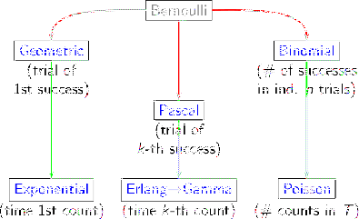
Here is, finally, a summary of the distributions
derived from the `apparently insignificant' Bernoulli process:
For completeness, let us also remind that:
- the famous
 distribution is technically a Gamma,
with
distribution is technically a Gamma,
with
 and
and  ;
;
- most distributions appearing in this scheme,
with the obvious exception of the geometric and the exponential,
which have fixed shape, `tend to a Gaussian distribution' for
some values of the parameters. In particular, for what concerns
this paper, the Poisson distribution tends to `normality' for `large'
values of
 , as well known. However, it is perhaps worth
remembering that, in general, such a limit applies
to the cumulative distribution,
and not to the probability function, defined for the Poisson
distribution only for non negative integers:
, as well known. However, it is perhaps worth
remembering that, in general, such a limit applies
to the cumulative distribution,
and not to the probability function, defined for the Poisson
distribution only for non negative integers:
 Poisson
![$\displaystyle (\lambda))\, \xrightarrow
[\,\ \lq \lambda\rightarrow \infty'\,\ ]{}
\,F(x\,\vert\,{\cal N}(\lambda,\sqrt{\lambda}))\,.$](img681.png)
![$\displaystyle \left(1-r\cdot \frac{t}{n}\right)^n
\xrightarrow[\ n\rightarrow\infty\ ]{}\, e^{-r\, t}\,.$](img635.png)