Next: Inferring numerical values of
Up: Bayesian inference for simple
Previous: Bayes' theorem
Making use of formulae (20) or (21), we can easily
solve many classical problems involving inference when many hypotheses
can produce the same single effect.
Consider the case of interpreting the results of a test for the
HIV virus applied to a randomly
chosen European. Clinical tests are very seldom perfect.
Suppose that the test accurately detects infection,
but has a false-positive rate of 0.2%:
If the test is positive, can we conclude that the particular person
is infected with a probability of 99.8%
because the test has only a 0.2% chance of mistake? Certainly not! This kind of mistake is often made by those who are not used to Bayesian reasoning, including scientists who make inferences in their own field of
expertise. The correct answer depends on
what we else know about the person tested, that is, the background information.
Thus, we have to consider the incidence of the HIV virus in Europe,
and possibly, information about the lifestyle of the individual.
For details, see (D'Agostini 1999c).
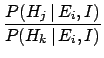
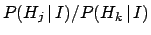
To better understand the updating mechanism, let us take the ratio of
Eq. (20) for two hypotheses  and
and 
where the sums in the denominators of Eq. (20) cancel.
It is convenient to interpret the ratio of probabilities,
given the same condition,
as betting odds. This is best done formally in
the de Finetti approach,
but the basic idea is what everyone is used to:
the amount of money that one is willing
to bet on an event is proportional to the degree to which
one expects that event will happen.
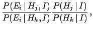
Equation (23) tells us that, when new
information is available, the initial odds are updated
by the ratio of the likelihoods
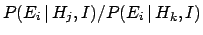 ,
which is known as
the Bayes factor.
,
which is known as
the Bayes factor.
In the case of the HIV test, the initial odds for an
arbitrarily chosen European to be infected
 are
so small that we need a very high Bayes' factor to
be reasonably certain that, when the test is positive, the person is
really infected.
With the numbers used in this example, the Bayes factor
is
are
so small that we need a very high Bayes' factor to
be reasonably certain that, when the test is positive, the person is
really infected.
With the numbers used in this example, the Bayes factor
is  . For example,
if we take for the prior
. For example,
if we take for the prior
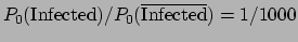 ,
the Bayes' factor changes these odds to
,
the Bayes' factor changes these odds to 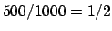 , or equivalently, the
probability that the person is infected would be
, or equivalently, the
probability that the person is infected would be  ,
quite different from the
,
quite different from the  answer usually prompted
by those who have a standard statistical education.
This example can be translated straightforwardly to physical problems,
like particle identification in the analysis of a Cherenkov detector
data, as done, e.g. in (D'Agostini 1999c).
answer usually prompted
by those who have a standard statistical education.
This example can be translated straightforwardly to physical problems,
like particle identification in the analysis of a Cherenkov detector
data, as done, e.g. in (D'Agostini 1999c).
Next: Inferring numerical values of
Up: Bayesian inference for simple
Previous: Bayes' theorem
Giulio D'Agostini
2003-05-13