|
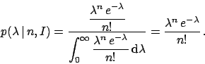
(43) |
When the observed value of ![]() is zero, Eq. (44)
yields
is zero, Eq. (44)
yields
![]() , giving a maximum of
belief at zero, but an exponential tail toward large values of
, giving a maximum of
belief at zero, but an exponential tail toward large values of
![]() . Expected value and standard deviation of
. Expected value and standard deviation of ![]() are both equal to 1.
The 95% probabilistic upper bound of
are both equal to 1.
The 95% probabilistic upper bound of ![]() is at
is at
![]() , as it can be easily calculated solving
the equation
, as it can be easily calculated solving
the equation
![]() .
Note that also this result depends on the
choice of prior, though Astone and D'Agostini (1999) have
shown that the upper bound is insensitive to
the exact form of the prior, if the prior models somehow what
they call ``positive attitude of rational scientists''
(the prior has not to be in contradiction with what one could actually observe,
given the detector sensitivity). In particular, they show that a uniform prior
is a good practical choice to model this attitude.
On the other hand, talking about `objective' probabilistic upper/lower
limits makes no sense, as discussed in detail and with examples in
the cited paper: one can at most
speak about conventionally defined non-probabilistic sensitivity bounds,
which separate the measurement region from that in which
experimental sensitivity is lost (Astone and D'Agostini 1999, D'Agostini 2000,
Astone et al 2002).
.
Note that also this result depends on the
choice of prior, though Astone and D'Agostini (1999) have
shown that the upper bound is insensitive to
the exact form of the prior, if the prior models somehow what
they call ``positive attitude of rational scientists''
(the prior has not to be in contradiction with what one could actually observe,
given the detector sensitivity). In particular, they show that a uniform prior
is a good practical choice to model this attitude.
On the other hand, talking about `objective' probabilistic upper/lower
limits makes no sense, as discussed in detail and with examples in
the cited paper: one can at most
speak about conventionally defined non-probabilistic sensitivity bounds,
which separate the measurement region from that in which
experimental sensitivity is lost (Astone and D'Agostini 1999, D'Agostini 2000,
Astone et al 2002).