Next: Reference priors
Up: General principle based priors
Previous: Transformation invariance
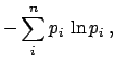
Maximum-entropy priors
Another principle-based approach to assigning priors
is based on in the Maximum Entropy principle
(Jaynes 1957a, also 1983, 1998, Tribus 1969, von der Linden 1995, Sivia
1997, and Fröhner 2000). The basic idea is to choose the prior
function that maximizes the
Shannon-Jaynes information entropy,
subject to whatever is assumed to be known about the distribution.
The larger  is, the greater
is our ignorance about the uncertain value of interest.
The value
is, the greater
is our ignorance about the uncertain value of interest.
The value  is obtained
for a distribution that concentrates all the probability into a single value.
In the case of no
constraint other than normalization, (
is obtained
for a distribution that concentrates all the probability into a single value.
In the case of no
constraint other than normalization, (
 ),
is maximized by the uniform
distribution,
),
is maximized by the uniform
distribution,  , which is easily proved using Lagrange multipliers.
For example, if the
variable is an integer between 0 and 10, a uniform distribution
, which is easily proved using Lagrange multipliers.
For example, if the
variable is an integer between 0 and 10, a uniform distribution
 gives
gives  .
Any binomial
distribution with
.
Any binomial
distribution with  gives a smaller value, with a maximum
of
gives a smaller value, with a maximum
of  for
for  and a
limit of for
and a
limit of for
 or or
or or
 ,
where
,
where  is now the parameter of the binomial that gives
the probability of success at each trial.
is now the parameter of the binomial that gives
the probability of success at each trial.
Two famous cases of maximum-entropy priors for continuous variables
are when the only information about
the distribution is either the expected value or the expected
value and the variance.
Indeed, these are special cases of general constraints
on the moments of the distribution  (see Tab. 1).
For
(see Tab. 1).
For  and 1, is equal to
unity and to the expected value, respectively. First and second moment
together provide the variance (see Tab. 1 and
Sect. 5.6). Let us sum up
what the assumed knowledge on the various moments provides
[see e.g. (Sivia 1997, Dose 2002)].
and 1, is equal to
unity and to the expected value, respectively. First and second moment
together provide the variance (see Tab. 1 and
Sect. 5.6). Let us sum up
what the assumed knowledge on the various moments provides
[see e.g. (Sivia 1997, Dose 2002)].
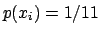
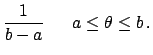
- Knowledge about

-
Normalization alone provides a uniform distribution over the interval
in which the variable is defined:
This is the extension to continuous variables
of the discrete case we saw above.
- Knowledge about and
 [i.e. about
 ]
]
-
Adding to the constraint  the knowledge about the
expectation of the variable, plus
the requirement that all non-negative values are allowed,
an exponential distribution is obtained:
the knowledge about the
expectation of the variable, plus
the requirement that all non-negative values are allowed,
an exponential distribution is obtained:
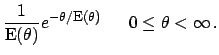
- Knowledge about , and
 [i.e. about
and
[i.e. about
and
 ]
]
-
Finally, the further constraint provided by the standard deviation (related to
first and second moment by the equation
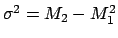 ) yields a prior
with a Gaussian shape independently of the range of , i.e.
) yields a prior
with a Gaussian shape independently of the range of , i.e.
The standard Gaussian is recovered when is
allowed to be any real number.
Note, however, that
the counterpart of
Eq. (105) for continuous variables is not trivial, since
all  of Eq. (105) tend to zero.
Hence the analogous functional form
of Eq. (105) tend to zero.
Hence the analogous functional form
 no longer has a sensible
interpretation in terms of uncertainty, as remarked
by Bernardo and Smith (1994).
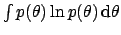
The Jaynes' solution is to introduce a `reference'
density
no longer has a sensible
interpretation in terms of uncertainty, as remarked
by Bernardo and Smith (1994).
The Jaynes' solution is to introduce a `reference'
density  to make entropy
invariant under coordinate transformation via
to make entropy
invariant under coordinate transformation via
![$\!\int p(\theta) \ln [p(\theta)/m(\theta)]\,\mbox{d}\theta$](img488.png) .
(It is important to remark that the first and the
third case discussed above are valid under the assumption
of a unity reference density.)
This solution is not universally
accepted (see Bernardo and Smith 1994), even though it conforms to the
requirements of dimensional analysis.
Anyhow, besides formal aspects and the undeniable aid of
Maximum Entropy methods in complicate problems such as
image reconstruction (Buck and Macauly 1991), we find it very
difficult, if not impossible at all, that a practitioner holds that
status of knowledge which give rise to the two celebrated
cases discussed above. We find more reasonable
the approach described in Sect. 8.2,
that goes the other way around:
we have a rough idea of where the quantity of interest
could be, then we try to model it and to summarize it
in terms of expected value and standard deviation. In particular, we find
untenable the position of those who state that
Gaussian distribution can only be justified by Maximum Entropy
principle.
.
(It is important to remark that the first and the
third case discussed above are valid under the assumption
of a unity reference density.)
This solution is not universally
accepted (see Bernardo and Smith 1994), even though it conforms to the
requirements of dimensional analysis.
Anyhow, besides formal aspects and the undeniable aid of
Maximum Entropy methods in complicate problems such as
image reconstruction (Buck and Macauly 1991), we find it very
difficult, if not impossible at all, that a practitioner holds that
status of knowledge which give rise to the two celebrated
cases discussed above. We find more reasonable
the approach described in Sect. 8.2,
that goes the other way around:
we have a rough idea of where the quantity of interest
could be, then we try to model it and to summarize it
in terms of expected value and standard deviation. In particular, we find
untenable the position of those who state that
Gaussian distribution can only be justified by Maximum Entropy
principle.
Next: Reference priors
Up: General principle based priors
Previous: Transformation invariance
Giulio D'Agostini
2003-05-13
![$\displaystyle \frac{\exp\left[-\frac{(\theta-\mbox{\footnotesize E}(\theta))^2}...
...\sigma^2(\theta)} \right]\,\mbox{d}\theta }
\hspace{0.6cm} a\le \theta \le b\,.$](img484.png)