An old Problem in the Doctrine of Chances

Evaluating the probability of future events on the basis of the outcomes of previous trials on `apparently the same conditions' is an old, classical problem in probability theory that goes back to about 250 years ago and it is associated to the names of Bayes [21] and Laplace [22]. The problem can be sketched as considering events whose probability of occurrence depends on a parameter which we generically indicate as $p$, i.e.

$$P(E\,\vert\,p) = p\,.$$

Idealized examples of the kind are the proportion of white balls in a box containing a large number of white and black balls (with the extracted ball put back into the box after each extraction), the bias of a coin and the ratio of the chosen surface in which a ball thrown `at random' can stop, with respect to the total surface of a horizontal table (this was the case of the Bayes' `billiard', although the Reverend did not mention a billiard).

A related problem concerns the number of times (`$X$') events of a given kind occur in $n$ trials, assuming that $p$ remains constant. The result is given by the well known binomial, that is

$$X \sim (n, p)\,,$$ (11)

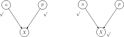
whose graphical causal model is shown in the left diagram of Fig. .

Figure: Graphical models of the binomial distribution (left) and its `inverse problem'. The symbol `$\surd$' indicates the `observed' nodes of the network, that is the value of the quantity associated to it is (assumed to be) certain. The other node (only one in this simple case) is `unobserved' and it is associated to a quantity whose value is uncertain.

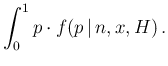
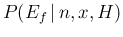
The problem first tackled in quantitative terms by Bayes and Laplace was how to evaluate the probability of a `future' event $E_f$, based on the information that in the past $n$ trials the event of that kind occurred $X=x$ times (`number of successes') and on the assumption of a regular flow from past to future,¹¹ that is assuming $p$ constant although uncertain. In symbols, we are interested in

$$P(E_f\,\vert\,n,x,H)\,,$$

where $H$ stands, as above, for all underlying hypotheses. Both Bayes and Laplace realized that the problem goes through two steps: first finding the probability distribution of $p$ and then evaluating $P(E_f\,\vert\,n,x,H)$ taking into account all possible values of $p$. In modern terms

$$1.\ \ \rightarrow \ \ \ \ f(p\,\vert\,n,x,H)$$ (12)

$$\ \ \ \ 2. \ \ \ \rightarrow \ P(E_f\,\vert\,n,x,H) = \int_0^1 \!P(E_f\,\vert\,p)\cdot f(p\,\vert\,n,x,H)$$ (13)

$$= \int_0^1 p \cdot f(p\,\vert\,n,x,H) \,.$$ (14)

The basic reasoning behind these two steps is expressly outlined in the Sixth and Seventh Principle of the Calculus of Probabilities, expounded by Laplace in Chapter III of his Philosophical Essay on Probabilities [23]:

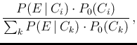
• the Sixth Principle, in terms of the possible causes $C_i$ responsible of the observed event $E$, is essentially what is presently known as Bayes' theorem, that is
  

  $$P(C_i\,\vert\,E) = \frac{P(E\,\vert\,C_i)\cdot P_0(C_i)} {\sum_k P(E\,\vert\,C_k)\cdot P_0(C_k)}\,,$$ (15)

  
  in which $P_0(C_i)$ is the so called prior probability of $C_i$, i.e. not taking into account the piece of information provided by the observation of $E$. Note that the role of $P_0(C_i)$ was explicitly considered by Laplace, who 1) before gave the rule in the case of $P_0(C_i)$ numerically all equal, which then drop from Eq. (); 2) then specified that “if these various causes, considered à priori, are unequally probable, it is necessary, in the place of the probability of the event resulting from each cause, to employ the product of this probability by the possibility of the cause itself.” (Here `possibility' and `probability' are clearly used as synonyms.) Then, the importance of the finding is stressed:

  “This is the fundamental principle of this branch of the analysis of chances which consists in passing from events to causes.”

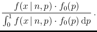
  Generalizing this `principle' to an infinite number of causes, associated to all possible values of the parameter $p$, with the `event' being the observation of $X=x$ successes in $n$ trials, we get the case sketched in the right diagram of Fig. , in which the unobserved node is now $p$. Equation () becomes then, in terms of the probability function of $X$ and of the pdf of $p$ $[$for which we take the freedom of using the same symbol `$f()$'$]$,
  

  $$f(p\,\vert\,n,x) = \frac{f(x\,\vert\,n,p)\cdot f_0(p)} {\int_0^1 f(x\,\vert\,n,p)\cdot f_0(p) \,\mbox{d}p}\,.$$ (16)

  
  
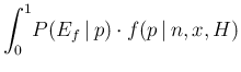
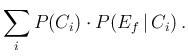
• The Seventh Principle then states that “the probability of a future event is the sum of the products of the probability of each cause, drawn from the event observed, by the probability that, this cause existing, the future event will occur”, that is
  

  $$P(E_f) = \sum_i P(C_i)\cdot P(E_f\,\vert\,C_i)\,.$$ (17)

  
  Generalizing also this `principle' to an infinite number of causes associated to all possible values of the parameter $p$ we get Eq. (), and then Eq. (): the probability of interest is the mean of the distribution of $p$.

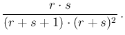
The solution of Eq. (), in the case $X$ is described by Eq. () and we consider all values of $p$ à priori equally likely, is a Beta pdf, that is¹²

$$p \sim (r,s)$$ (18)

with $r=x+1$ and $s=n-x+1$. Mean value and variance of the possible values of $p$ are then

$$\mu \equiv (p) = \frac{r}{r+s}$$ (19)

$$\sigma^2 \equiv (p) = \frac{r\cdot s}{(r+s+1)\cdot(r+s)^2}\,.$$ (20)

Finally, using Eq. () and Eq. () we get the Laplace's rule of succession

$$P(E_f\,\vert\,n,x,H) = \frac{x+1}{n+2}\,.$$ (21)

Thus, in the special case of `$n$ successes in $n$ trials', “we find that an event having occurred successively any number of times, the probability that it will happen again the next time is equal to this number increased by unity divided by the same number, increased by two units” [23], i.e.

$$P(E_f\,\vert\,n,x=n,H) = \frac{n+1}{n+2}\,.$$ (22)

In the case of $x=n=11$ we have then 12/13, or 92.3%. Reporting thus 100% (see footnote ) can be at least misleading, especially because such a value can be (as it has indeed been) nowadays promptly broadcasted uncritically by the media (see e.g. [16] - we have heard so far no criticism in the media of such an incredible claim, but only sarcastic comments by colleagues).