- ...
causes.1
- One might object that if the same cause yields
different effects in different trials, then other concauses must exist,
responsible for the differentiation of the effects.
This point of view leads e.g. to the `hidden variables' interpretation
of quantum mechanics (`à la Einstein').
I have no intention to try to solve, or even to touch all philosophical
questions related to causation (for a modern and fruitful approach,
see Ref. [2] and references therein)
and of the fundamental aspects of
quantum mechanics.
The approach followed here
is very pragmatic and the concept of causation is, to say,
a weak one,
that perhaps could be better called conditionalism:
``whenever I am sure of this, then I am
also somehow confident that that will occur''.
The degree of confidence on the occurrence of that
might rise from past experience, just from reasoning,
or from both.
It is not really relevant whether
this is the cause of that in a classical sense,
or this and that are both due to other `true causes'
and we only perceive a correlation between this and that.
.
.
.
.
.
.
.
.
.
.
.
.
.
.
.
.
.
.
.
.
.
.
.
.
.
.
.
.
.
.
- ... proceeds,2
- Those who believe that
scientists are really `falsificationist' can find enlighting
the following famous Einstein's quote:
``If you want to find out anything from
the theoretical physicists about the methods they use,
I advise you to stick closely to one principle:
don't listen to their words, fix your attention
on their deeds.''[6]. We shall come to this point
in the conclusions.
.
.
.
.
.
.
.
.
.
.
.
.
.
.
.
.
.
.
.
.
.
.
.
.
.
.
.
.
.
.
- ...
impossible'.3
- In the hypothetical experiment of
one million tosses of a hypothetical `regular coin'
(easily realized by a little simulation)
the result of 500000 heads
represents an `extraordinary event' (
 probability),
as `extraordinary' are all other possible outcomes!
probability),
as `extraordinary' are all other possible outcomes!
.
.
.
.
.
.
.
.
.
.
.
.
.
.
.
.
.
.
.
.
.
.
.
.
.
.
.
.
.
.
- ...
Logically,4
- The fact that in practice these methods `often work'
is a different story, as discussed in Sec. 10.8 of Ref. [1].
.
.
.
.
.
.
.
.
.
.
.
.
.
.
.
.
.
.
.
.
.
.
.
.
.
.
.
.
.
.
- ... observed5
- In other words,
the reasoning based on p-values [8]
constantly violates the so called likelihood principle,
apart from exceptions due to
numerical coincidences. In fact, making the
simple example of a single-tail
test based on a variable that is indeed observed, the
conclusion about acceptance or rejection is made on the basis of
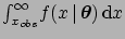 ,
where
,
where
 are the model parameters.
But this integral is rarely simply proportional
to the likelihood
are the model parameters.
But this integral is rarely simply proportional
to the likelihood
 , i.e. integral and likelihood
do not differ
by just a constant factor not depending on
.
I would like to make clear that I dislike
un-needed principles,
including the likelihood one,
and the maximum likelihood one above all.
The reason why I refer here to the likelihood principle in my argumentation
is that, generally, frequentists consider this principle with
some respect, but their methods usually violate it [9].
Instead, in the probabilistic approach illustrated in the sequel,
this 'principle' stems automatically from the theory.
, i.e. integral and likelihood
do not differ
by just a constant factor not depending on
.
I would like to make clear that I dislike
un-needed principles,
including the likelihood one,
and the maximum likelihood one above all.
The reason why I refer here to the likelihood principle in my argumentation
is that, generally, frequentists consider this principle with
some respect, but their methods usually violate it [9].
Instead, in the probabilistic approach illustrated in the sequel,
this 'principle' stems automatically from the theory.
.
.
.
.
.
.
.
.
.
.
.
.
.
.
.
.
.
.
.
.
.
.
.
.
.
.
.
.
.
.
- ...
construction.6
- In statistics the variables that
summarize all the information sufficient for the inference
are called a sufficient statistics (classical
examples are the sample average and standard deviation to infer
 and
and  of a Gaussian distribution).
However, I do not know of test variables that
can be considered sufficient for hypothesis tests.
of a Gaussian distribution).
However, I do not know of test variables that
can be considered sufficient for hypothesis tests.
.
.
.
.
.
.
.
.
.
.
.
.
.
.
.
.
.
.
.
.
.
.
.
.
.
.
.
.
.
.
- ...
calculated.7
- Imagine you have to decide if the extraction of
 white balls in
 trials can be considered in agreement with the hypothesis
that the box contains a given percentage
trials can be considered in agreement with the hypothesis
that the box contains a given percentage  of
white balls. You might think that
you are dealing with a binomial problem,
in which plays the role of random variable,
calculate the p-value and draw your conclusions.
But you might get the information that
the person who made the extraction had decided to
go on until he/she reached
white balls. In this case
the random variable is , the problem is modeled
by a Pascal distribution (or, alternatively, by a negative
binomial in which the role of random variable is played
by the number
of
white balls. You might think that
you are dealing with a binomial problem,
in which plays the role of random variable,
calculate the p-value and draw your conclusions.
But you might get the information that
the person who made the extraction had decided to
go on until he/she reached
white balls. In this case
the random variable is , the problem is modeled
by a Pascal distribution (or, alternatively, by a negative
binomial in which the role of random variable is played
by the number  of non-white balls)
and the evaluation of the p-value differs
from the previous one. This problem is known as the stopping rule problem.
It can be proved that the likelihood calculated from the two reasonings
differ only by a constant factor, and hence the likelihood principle
tells that the two reasonings should lead to identical inferential conclusions
about the unknown percentage of white balls.
of non-white balls)
and the evaluation of the p-value differs
from the previous one. This problem is known as the stopping rule problem.
It can be proved that the likelihood calculated from the two reasonings
differ only by a constant factor, and hence the likelihood principle
tells that the two reasonings should lead to identical inferential conclusions
about the unknown percentage of white balls.
.
.
.
.
.
.
.
.
.
.
.
.
.
.
.
.
.
.
.
.
.
.
.
.
.
.
.
.
.
.
- ... behaviors.8
- Just in this workshop I have
met yet another invention [10]:
Given three model fits to data with
40 degrees of freedom and the three
resulting
 of 37.9, 49.1 and 52.4 for
models
of 37.9, 49.1 and 52.4 for
models  ,
,  and , the common frequentistic wisdom
says the three models are about equivalent in describing the data,
because the expected is
and , the common frequentistic wisdom
says the three models are about equivalent in describing the data,
because the expected is  , or that none of the models
can be ruled out because all p-values
(0.56, 0.15 and 0.091, respectively) are above the usual
critical level of significance.
Nevertheless, SuperKamiokande claims that models
, or that none of the models
can be ruled out because all p-values
(0.56, 0.15 and 0.091, respectively) are above the usual
critical level of significance.
Nevertheless, SuperKamiokande claims that models  and are
`disfavored' at 3.3 and 3.8 's, respectively! (
and are
`disfavored' at 3.3 and 3.8 's, respectively! (
 and
and
 probability.) It seems
the result has been achieved using
inopportunely a technique of parametric inference. Imagine a minimum
fit of the parameter
probability.) It seems
the result has been achieved using
inopportunely a technique of parametric inference. Imagine a minimum
fit of the parameter  for which the data
give a minimum
of 37.9 at
for which the data
give a minimum
of 37.9 at
 , while
 and
and
 (and the curve is parabolic).
It follows that
(and the curve is parabolic).
It follows that  and
and  are, respectively,
 's and
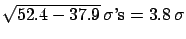 's far
from
's far
from  . The probability
that differs from by more than
. The probability
that differs from by more than
 and
and
 is then
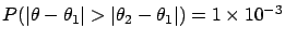 and
and
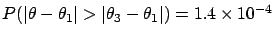 ,
respectively.
But this is quite a different problem!
,
respectively.
But this is quite a different problem!
.
.
.
.
.
.
.
.
.
.
.
.
.
.
.
.
.
.
.
.
.
.
.
.
.
.
.
.
.
.
- ...ADD.9
- Reference [11] has to be taken
more for its methodological contents than
for the physical outcome (a tiny piece of evidence in favor
of the searched for signal),
for in the meanwhile I have
become personally very sceptical about the experimental
data on which the analysis was based,
after having heard a couple of public talks by authors of those data
during 2004 (one in this workshop).
.
.
.
.
.
.
.
.
.
.
.
.
.
.
.
.
.
.
.
.
.
.
.
.
.
.
.
.
.
.