The pattern
 of
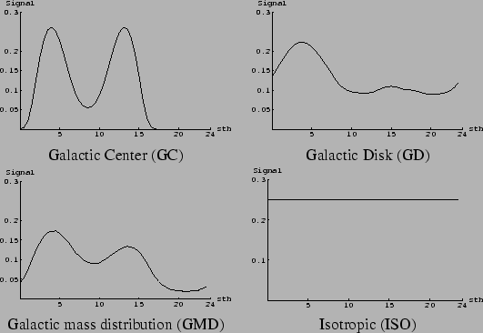
the two detectors Explorer and Nautilus to signals due to these
models are shown in Fig. 2.
These patterns are all given as a function of the sidereal time.
of
the two detectors Explorer and Nautilus to signals due to these
models are shown in Fig. 2.
These patterns are all given as a function of the sidereal time.
![]() depends on the space
and energy distributions of g.w. sources described by a model, taking
also into account the variation of the
detector efficiency with the sidereal time, due to the varying orientation
of the antennae respect to the sources. It depends also
on the (unknown) energies of g.w.
signals, on the noise, and on the coordinates (latitude,longitude,azimuth)
of the detectors on Earth.
Simply speaking, for various models of
the space distribution of sources of g.w.,
we expect different responses from the
coincidence experiment, i.e. different `antenna patterns',
seen as a function of the sidereal time.
depends on the space
and energy distributions of g.w. sources described by a model, taking
also into account the variation of the
detector efficiency with the sidereal time, due to the varying orientation
of the antennae respect to the sources. It depends also
on the (unknown) energies of g.w.
signals, on the noise, and on the coordinates (latitude,longitude,azimuth)
of the detectors on Earth.
Simply speaking, for various models of
the space distribution of sources of g.w.,
we expect different responses from the
coincidence experiment, i.e. different `antenna patterns',
seen as a function of the sidereal time.
The calculation of
![]() depends on the expected g.w. energy
and some assumptions are needed.
The signal's amplitude
depends on the expected g.w. energy
and some assumptions are needed.
The signal's amplitude ![]() is unknown, and thus we have evaluated the
patterns by integrating over a uniform distribution of
is unknown, and thus we have evaluated the
patterns by integrating over a uniform distribution of ![]() values,
ranging - on Earth - from
values,
ranging - on Earth - from
![]() up to
up to
![]() .
Different reasonings may be done here, leading to
different choices for the amplitudes range and for the distributions of the signals.
We have done the simplest choice, supposing that we do not know
anything on the signals, but the fact that no signals
have been observed at the detectors with amplitude greater than
.
Different reasonings may be done here, leading to
different choices for the amplitudes range and for the distributions of the signals.
We have done the simplest choice, supposing that we do not know
anything on the signals, but the fact that no signals
have been observed at the detectors with amplitude greater than
![]() .
The lowest limit has been
chosen considering the fact that the detector's efficiencies below
.
The lowest limit has been
chosen considering the fact that the detector's efficiencies below
![]() is very small (less than
is very small (less than
![]() ).
Note that the considered
).
Note that the considered ![]() values
are based on `standard' assumptions about the
g.w. energy release in cryogenic bars.
The Galactic Disk (GD) model has been constructed considering g.w. sources
uniformly distributed over the Galactic plane, which means a distribution of
sources which is not uniform around
the Earth, given the fact that the Earth is
values
are based on `standard' assumptions about the
g.w. energy release in cryogenic bars.
The Galactic Disk (GD) model has been constructed considering g.w. sources
uniformly distributed over the Galactic plane, which means a distribution of
sources which is not uniform around
the Earth, given the fact that the Earth is ![]() kpc from the Center of
Galaxy, which is the center of the disk (whose radius is
kpc from the Center of
Galaxy, which is the center of the disk (whose radius is ![]() kpc).
The GMD distribution, taking into account the mass distribution in Galaxy,
is much more interesting than the GD model. In fact we do not expect
a uniform distribution of the sources over the GD, but a distribution which is
concentrated near the GC [7].
kpc).
The GMD distribution, taking into account the mass distribution in Galaxy,
is much more interesting than the GD model. In fact we do not expect
a uniform distribution of the sources over the GD, but a distribution which is
concentrated near the GC [7].