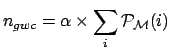
| (11) |
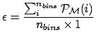
 is the ``overall efficiency of detection'',
 | (13) |
 |
(15) |
 . It can be
said, in simple words, to be the number of g.w. events
that could be present in each bin
in a coincidence experiment having
performance and exposure time as that described in Ref. [1].
Hence,
. It can be
said, in simple words, to be the number of g.w. events
that could be present in each bin
in a coincidence experiment having
performance and exposure time as that described in Ref. [1].
Hence,
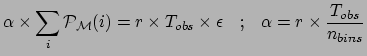
| (16) |
 and the rate
 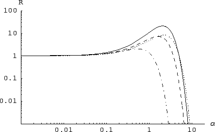 's are shown in Fig. 3.
Note that the figures are in log-log scale to make it clear that many
orders of magnitude of
's are shown in Fig. 3.
Note that the figures are in log-log scale to make it clear that many
orders of magnitude of
The results are summarized in
Tab. 1.
| Model | GC | GD | GMD | ISO |
|
|
4.7 | 6.1 | 4.4 | 12 |
| (%) |
9.8 | 13 | 9.2 | 25 |
|
|
21 | 7.2 | 8.2 | 1.9 |
| (events) | ||||
|
|
2.1 | 1.6 | 2.2 | 0.5 |
|
|
1.0 | 0.9 | 1.2 | 0.5 |
| E
|
2.3 | 1.8 | 2.5 | 0.7 |
|
|
1.0 | 0.9 | 1.2 | 0.4 |
| (events) | ||||
|
|
10 | 10 | 10 | 7 |
|
|
5 | 5 | 5 | 6 |
| E
|
11 | 11 | 11 | 9 |
|
|
5 | 6 | 5 | 5 |
| (events/day) | ||||
| 1.1 | 0.9 | 1.2 | 0.3 | |
|
|
0.5 | 0.5 | 0.7 | 0.3 |
| E
|
1.2 | 1.0 | 1.3 | 0.4 |
|
|
0.6 | 0.5 | 0.6 | 0.2 |
Figure 3 shows clearly how the initial beliefs about ![]() (and therefore on
(and therefore on ![]() )
are updated, within each model. We want to stress that
the final conclusion depends still on the prior beliefs.
If someone thought that
)
are updated, within each model. We want to stress that
the final conclusion depends still on the prior beliefs.
If someone thought that ![]() had to be above 10
this person had to reconsider completely his/her beliefs,
independently from the model;
if another person believed that only values below 0.01 were
reasonable,
the experiment would not affect at all his/her beliefs,
independently of the model. For this reason, the ML value
had to be above 10
this person had to reconsider completely his/her beliefs,
independently from the model;
if another person believed that only values below 0.01 were
reasonable,
the experiment would not affect at all his/her beliefs,
independently of the model. For this reason, the ML value
![]() could be misleading if erroneously associated,
as it often happens, to the value around which our confidence is
finally concentrated, independently from any prior knowledge.
Nevertheless, and with these warnings,
we report in Tab. 1 also the results obtained
from a ML analysis and from a
naïve Bayesian inference that assumes a uniform prior on
could be misleading if erroneously associated,
as it often happens, to the value around which our confidence is
finally concentrated, independently from any prior knowledge.
Nevertheless, and with these warnings,
we report in Tab. 1 also the results obtained
from a ML analysis and from a
naïve Bayesian inference that assumes a uniform prior on ![]() (and therefore on
(and therefore on ![]() and , since they differ by factors).
and , since they differ by factors).
![]() has been evaluated from the curvature of
the minus-log-likelihood around its minimum, i.e.
has been evaluated from the curvature of
the minus-log-likelihood around its minimum, i.e.
![]()
![]() .
The results of the `naïve Bayesian inference' are reported
as expected values E
.
The results of the `naïve Bayesian inference' are reported
as expected values E![]() and standard deviations evaluated
from the final distribution. The condition
and standard deviations evaluated
from the final distribution. The condition
![]() has
been written explicitly in E
has
been written explicitly in E![]() and
and
![]() , according to the Bayesian spirit.
Note that, for obvious reasons, the mode of
the posterior calculated using a uniform prior is exactly equivalent
to the ML estimate. This observation is important
to understand the slightly different results obtained with the
two methods. The posterior expected value is always larger
than the ML one, simply because of the asymmetry of
, according to the Bayesian spirit.
Note that, for obvious reasons, the mode of
the posterior calculated using a uniform prior is exactly equivalent
to the ML estimate. This observation is important
to understand the slightly different results obtained with the
two methods. The posterior expected value is always larger
than the ML one, simply because of the asymmetry of ![]() .
.
Perhaps is the most interesting quantity to understand
the conclusions of these
model dependent
analyzes that, we like to repeat it,
do not take properly into account prior knowledge.
The three physical model suggest about 10 coincidences
due to g.w.'s, with a 50% uncertainty. Instead,
for the unphysical model (ISO)
less events are found and with larger uncertainty. Note that, for this model,
the mode
of the posterior (or, equivalently, the ![]() estimate) gives a number
of candidate events that is the difference between the total number of
observed events
and that expected from the background alone. Instead, for the three
Galactic models, a number of events larger than this difference is
attributed to the signal, as a consequence of a `possibly good'
time modulation recognized in the data
(in other words, the method `likes to think' that, given
a time distribution shape that reminds the pattern of the Galactic models,
the background has most likely under-fluctuated within what is reasonably
allowed by its probability distribution).
estimate) gives a number
of candidate events that is the difference between the total number of
observed events
and that expected from the background alone. Instead, for the three
Galactic models, a number of events larger than this difference is
attributed to the signal, as a consequence of a `possibly good'
time modulation recognized in the data
(in other words, the method `likes to think' that, given
a time distribution shape that reminds the pattern of the Galactic models,
the background has most likely under-fluctuated within what is reasonably
allowed by its probability distribution).
To summarize this subsection,
the three Galactic
models show good agreement in indicating for which values of
g.w. events, or event rate, we must increase our beliefs.
But the final beliefs depend on our initial ones,
as explained introducing the Bayesian approach.
If you think that, given your best knowledge of the models of g.w.'s sources and
of g.w. interaction with cryogenic detectors, a g.w. rate on Earth of
up to
![]() event/day is quite possible, the data make you
to believe that this rate is
event/day is quite possible, the data make you
to believe that this rate is
![]() event/day
and that they contain
event/day
and that they contain
![]() genuine g.w. coincidences.
genuine g.w. coincidences.