While in the previous subsection we have been interested to learn about ![]() or
or ![]() within a model (and then, since all results are conditioned by that
model, it makes no sense from that perspective to state if the model is
right or wrong), let us see now how to modify our beliefs on each
model.
This is a delicate question to be treated
with care. Intuitively, we can imagine that we have to
make use of the
within a model (and then, since all results are conditioned by that
model, it makes no sense from that perspective to state if the model is
right or wrong), let us see now how to modify our beliefs on each
model.
This is a delicate question to be treated
with care. Intuitively, we can imagine that we have to
make use of the ![]() values, in the sense that
the higher is the value and the most `the hypothesis'
increases its credibility. The crucial point is to understand that
`the hypothesis' is, indeed, a complex (somewhat multidimensional)
hypothesis. Another important point is that, given a non null background
and the properties of the Poisson distribution,
we are never certain that the
observations are not due to background alone (this is
the reason why the
values, in the sense that
the higher is the value and the most `the hypothesis'
increases its credibility. The crucial point is to understand that
`the hypothesis' is, indeed, a complex (somewhat multidimensional)
hypothesis. Another important point is that, given a non null background
and the properties of the Poisson distribution,
we are never certain that the
observations are not due to background alone (this is
the reason why the ![]() function does not
vanish for
function does not
vanish for
![]() ).
).
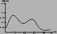
The first point can be well understood making an example based
on Fig. 3 and Tab. 1.
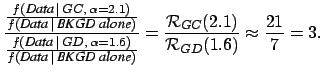
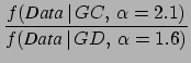
Comparing
![]() for the different models one could come
to the rash conclusion that the Galactic Center model is enhanced by
21 with respect to the non g.w. hypothesis, or that
the Galactic Center model is enhanced by a factor
for the different models one could come
to the rash conclusion that the Galactic Center model is enhanced by
21 with respect to the non g.w. hypothesis, or that
the Galactic Center model is enhanced by a factor ![]() with respect to the hypothesis of signals
from sources uniformly distributed over the Galactic Disk.
However these conclusions would be correct only in the case that each
model would admit only that value of the parameter which
maximizes
with respect to the hypothesis of signals
from sources uniformly distributed over the Galactic Disk.
However these conclusions would be correct only in the case that each
model would admit only that value of the parameter which
maximizes ![]() , i.e.
, i.e.
 and not in
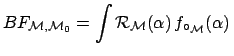
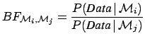
Let us take the Bayes factor defined in Eq. (7). The probability theory teaches us promptly what to do when each model depends on parameters:
 |
(18) |
To better understand the role of the parameter prior
in Eq. (21), let us take the example of a model
(which we do not consider realistic and, hence, we have discarded
a priori in our analysis) that gives a signal only in one of the 1/2 hours bins,
being all bins a priori equally possible.
This model
![]() would depend on two parameters,
would depend on two parameters, ![]() and
and ![]() ,
where
,
where ![]() is the center of the time bin. Considering
is the center of the time bin. Considering ![]() and
and ![]() independent,
the parameter prior is
independent,
the parameter prior is
![]() ,
where
,
where
![]() is a probability function for the discrete variable
is a probability function for the discrete variable
![]() . The `evidence' for this model would be
. The `evidence' for this model would be
 d
d d
d
 d
d
 with respect to other models that do not have the time position
as free parameter. Note that this suppression
goes in the same direction
of the reasoning described in Sec. 3.3.
But the Bayesian approach tells us when and how this suppression
has to be applied. Certainly not in the Galactic models we are considering.
with respect to other models that do not have the time position
as free parameter. Note that this suppression
goes in the same direction
of the reasoning described in Sec. 3.3.
But the Bayesian approach tells us when and how this suppression
has to be applied. Certainly not in the Galactic models we are considering.
As we have seen, while the Bayes factors for simple hypotheses
(`simple' in the sense that they have no internal parameters)
provide a prior-free information of how to modify the beliefs,
in the case of models with free parameters Bayes factors
remain independent from the beliefs about the models, but do depend
on the priors about the model parameters. In our case they depend
on the priors about ![]() , which might be different for different
models. If we were comparing different models,
each with its
, which might be different for different
models. If we were comparing different models,
each with its
![]() about which there is full agreement
in the scientific community, all further calculations would be
straightforward. However, we do not think to be in such a nice
text-book situation, dealing with open problems in frontier physics
(for example, note that
about which there is full agreement
in the scientific community, all further calculations would be
straightforward. However, we do not think to be in such a nice
text-book situation, dealing with open problems in frontier physics
(for example, note that ![]() , and then
, and then ![]() and
and 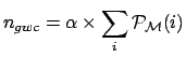 , depend on
the g.w. cross section on cryogenic bars, and we do not believe
that the understanding of the underlying mechanisms is completely settled).
In principle every physicist which have formed his/her ideas
about some model and its parameters should insert his/her functions
in the formulae and see from the result how he/she should change
his/her opinion about the different models.
Virtually our task ends here,
having given the
, depend on
the g.w. cross section on cryogenic bars, and we do not believe
that the understanding of the underlying mechanisms is completely settled).
In principle every physicist which have formed his/her ideas
about some model and its parameters should insert his/her functions
in the formulae and see from the result how he/she should change
his/her opinion about the different models.
Virtually our task ends here,
having given the ![]() functions, which can be seen as the
best summary of an experimental fact, and having indicated how to proceed
(for recent examples of applications of this method in astrophysics and cosmology
see Refs. [10,11,12]).
Indeed, we proceed,
showing how beliefs can change given some possible scenarios for
functions, which can be seen as the
best summary of an experimental fact, and having indicated how to proceed
(for recent examples of applications of this method in astrophysics and cosmology
see Refs. [10,11,12]).
Indeed, we proceed,
showing how beliefs can change given some possible scenarios for
![]() .
.
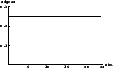
The first scenario is that in which
the possible value of ![]() are considered so small that
are considered so small that
![]() is equal to zero for
is equal to zero for
![]() .
The result is simple: the data are irrelevant and beliefs
on the different models are not updated by the data.
.
The result is simple: the data are irrelevant and beliefs
on the different models are not updated by the data.
Other scenarios might allow
the possibility that
![]() is positive for values up to
is positive for values up to
![]() and more. We shall use
three different pdf's for
and more. We shall use
three different pdf's for ![]() as examples of prior beliefs,
that we call `sceptical', `moderate' and 'uniform' (up to
as examples of prior beliefs,
that we call `sceptical', `moderate' and 'uniform' (up to ![]() ).
The `moderate' pdf corresponds to a rate
which is rapidly going to zero around the value which we have measured.
The initial pdf is modeled with a half-Gaussian with
).
The `moderate' pdf corresponds to a rate
which is rapidly going to zero around the value which we have measured.
The initial pdf is modeled with a half-Gaussian with ![]() .
The `sceptical' pdf has a
.
The `sceptical' pdf has a ![]() ten times smaller.
The `uniform' considers equally likely
all
ten times smaller.
The `uniform' considers equally likely
all ![]() up to the last decade
in which the
up to the last decade
in which the ![]() functions are sizable different from zero.
Here are the three
functions are sizable different from zero.
Here are the three
![]() :
:
| (22) | |||
| (23) | |||
| (24) |
Using these three pdf's for the parameter ![]() ,
we can finally calculate all Bayes factors.
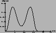
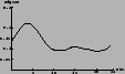
We report in Tab. 2 the Bayes factors of the models
of Fig. 2 with respect to model
,
we can finally calculate all Bayes factors.
We report in Tab. 2 the Bayes factors of the models
of Fig. 2 with respect to model
![]() ``only background'',
using Eq. (20).
All other Bayes factors can be calculated as ratio of these.
``only background'',
using Eq. (20).
All other Bayes factors can be calculated as ratio of these.
| `sceptical' | `moderate' | `uniform' | |
|
|
 |
|
|
|
|
1.3 | 8.4 | 5.4 |
 |
1.4 | 4.1 | 1.7 |
 |
1.2 | 3.9 | 2.6 |
 |
1.2 | 1.4 | 0.2 |
 event/day),
then Bayes factors are obtained
which that can sizable increase our suspicion that some events could be really due
to one of these models.1Within this `moderate' scenario there is some preference for the Galactic Center model
with a Bayes factor about 2 with respect to each other model. This result
contradict the naïve judgment based on observation of a `peak' at
around 4:00. The response of the Bayesian comparison takes into account
all features of the model pattern, including the width of the peaks.
event/day),
then Bayes factors are obtained
which that can sizable increase our suspicion that some events could be really due
to one of these models.1Within this `moderate' scenario there is some preference for the Galactic Center model
with a Bayes factor about 2 with respect to each other model. This result
contradict the naïve judgment based on observation of a `peak' at
around 4:00. The response of the Bayesian comparison takes into account
all features of the model pattern, including the width of the peaks.
We have also considered a prior which is uniform in
![]() , between
, between
![]() .
This prior accords equal probability to each decade in the parameter
.
This prior accords equal probability to each decade in the parameter ![]() , and probably
accords many people prior intuition.
Bayes factors, for the four models of Fig. 2
with respect to model
, and probably
accords many people prior intuition.
Bayes factors, for the four models of Fig. 2
with respect to model
![]() ``only background'', are:
``only background'', are:
4.0 (GC); 2.0 (GD); 2.2 (GMD); 1.0 (ISO).
Again, within this scenario there is some preference for the Galactic Center model with a Bayes factor about 2 with respect to each other model.
 d
d