This paper is mainly on methodological issues related to model comparisons in critical, frontier physics cases where the prior knowledge is relevant.
We have given reasons of why `conventional statistics' (i.e. the collection of frequentistic prescriptions) does not adequately approach the problem of model comparison, mainly because of impossibility of classify hypotheses in a probability scale and of the pretension that good criteria to state what is `significant' can be derived from the properties of the null hypothesis alone, without considering the details of the alternative hypotheses.2
Within the so called Bayesian framework, we have
started from the basic observation
that the most a probability theory
should do is to provide
rules to modify our beliefs on the light of experimental data.
Beliefs can be about the values of the parameters of a model or
about alternative models. As far as beliefs on model parameters
are concerned, we have shown that the likelihood, rescaled to its
insensitivity limit value (the ![]() function,
or `relative belief
updating factor'), represents
a good, prior independent way of summarizing the information
contained in the data with respect to a given model.
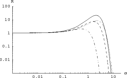
Indeed, when this method is applied to the Explorer-Nautilus data,
from the visual inspection of the
function,
or `relative belief
updating factor'), represents
a good, prior independent way of summarizing the information
contained in the data with respect to a given model.
Indeed, when this method is applied to the Explorer-Nautilus data,
from the visual inspection of the ![]() function
the reader gets, for each model, an immediate
overview of what the data say about
the number of events involved in the observation.
The
function
the reader gets, for each model, an immediate
overview of what the data say about
the number of events involved in the observation.
The ![]() values for which the relative belief
updating factor is maximum correspond to a total number of
g.w. events in the data (
values for which the relative belief
updating factor is maximum correspond to a total number of
g.w. events in the data (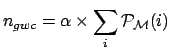 ) about 10 for all three Galactic
models. For those who share beliefs
that numbers of this order
of magnitude or more are possible
(and that one of the three models is the correct one),
the
) about 10 for all three Galactic
models. For those who share beliefs
that numbers of this order
of magnitude or more are possible
(and that one of the three models is the correct one),
the ![]() can be translated
into a result
can be translated
into a result
![]() (or a rate on Earth of
(or a rate on Earth of
![]() ).
).
Going to the model comparison, we have shown the unavoidable complication
due to the fact that each model depends on a free parameter (![]() )
and, hence, the Bayes factors depend on the prior pdf of this parameter,
i.e.
)
and, hence, the Bayes factors depend on the prior pdf of this parameter,
i.e.
![]() .
Since the models used do not come with a kind of reference
.
Since the models used do not come with a kind of reference
![]() (we hope that more work will be done in this direction)
we had to do some choices and we have given the results under
different scenarios, from the most negative one (``there is no chance that
the models produce something observable, given the present energy
sensitivity'') to some others in which
(we hope that more work will be done in this direction)
we had to do some choices and we have given the results under
different scenarios, from the most negative one (``there is no chance that
the models produce something observable, given the present energy
sensitivity'') to some others in which ![]() above 1
are conceivable (described by the priors
we have called in the text `moderate' and 'uniform'). Given these
scenarios the Galactic Center model gets preferred
over the others by a Bayes factor of about 2:1.
above 1
are conceivable (described by the priors
we have called in the text `moderate' and 'uniform'). Given these
scenarios the Galactic Center model gets preferred
over the others by a Bayes factor of about 2:1.
We would like to end replying to the objection, arisen often in discussions, that ``the plot with coincidences grouped in bins of sidereal time provides the same information of that in which coincidences are grouped in bins of solar time''. This might be true if one is blindly looking for ``statistical significance'', following strictly frequentistic prescriptions, which, as explained above, we do not consider the proper way to go.
To answer this objection we have done the exercise of applying exactly the same analysis with the same models to the data grouped in bins of solar time.
| `sceptical' | `moderate' | `uniform' | |
|
|
 |
|
|
|
|
1.0 | 0.5 | 0.1 |
 |
1.1 | 1.2 | 0.3 |
 |
1.0 | 0.9 | 0.2 |
 |
1.2 | 1.2 | 0.2 |
 depend on the individual occurrence of the multinomial data set
(but never forget that the multinomial distribution does not
forbid strong clustering of the entries around one bin!).
depend on the individual occurrence of the multinomial data set
(but never forget that the multinomial distribution does not
forbid strong clustering of the entries around one bin!).
The lesson from this exercise is that the Explorer-Nautilus 2001 data, plotted as a function of a sensible physical quantity and compared with physically motivated models, does not provide the same information of any random sample. Indeed, the evidence in support of the models is not enough to modify strongly our beliefs, but it is certainly at the level of ``stay tuned'', waiting for results of the 2003 run.