- ...
formulas1
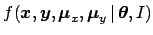
- The meaning of the overall conditioning
 will be clarified later. Note that,
in order to simplify the notation, the generic
symbol
will be clarified later. Note that,
in order to simplify the notation, the generic
symbol  is used to indicate all probability density functions,
though they might
refer to different variables and have different mathematical
expressions.
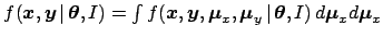
In particular, the order of the arguments is irrelevant,
in the sense that
is used to indicate all probability density functions,
though they might
refer to different variables and have different mathematical
expressions.
In particular, the order of the arguments is irrelevant,
in the sense that  stands for `joint probability density function
of
stands for `joint probability density function
of  and
and  under condition ',
and therefore it could be also indicated by
under condition ',
and therefore it could be also indicated by  .
For the same reason, the indexes of sums and products and
the extremes of the integrals
are usually omitted, implying they extend
to all possible values of the variables.
.
For the same reason, the indexes of sums and products and
the extremes of the integrals
are usually omitted, implying they extend
to all possible values of the variables.
.
.
.
.
.
.
.
.
.
.
.
.
.
.
.
.
.
.
.
.
.
.
.
.
.
.
.
.
.
.
- ... quantities2
- These quantities might also be
summaries of the data. I.e. they are either directly observed numbers,
like readings on scales, or quantities calculated from direct observations,
like averages or other `statistics' based on partial analysis of the data.
It is implicit that when summaries are used, instead of direct observations,
the analyzer is somewhat relying on the so called 'statistical sufficiency'.
.
.
.
.
.
.
.
.
.
.
.
.
.
.
.
.
.
.
.
.
.
.
.
.
.
.
.
.
.
.
- ...
problem,3
- Priors need to be specified for the nodes
of a Bayesian network that have no parents
(see Fig 1 and footnote 4).
Priors
are logically necessary ingredients, without
which probabilistic inference is simply impossible.
I understand that those who approach
this kind of reasoning for the first time
might be scared of this `subjective ingredient',
and because of it
they might prefer methods advertised as `objective'
to which they are used, formally not depending on priors.
However, if one thinks a bit deeper to the question,
one realizes that behind the slogan of `objectivity'
there is much arbitrariness,
of which the users are often not aware, and that might lead to
seriously wrong results in critical problems. Instead, the Bayesian approach
offers the logical tool to properly
blend prior judgment
and empirical evidence. For further comments see Ref. [2],
where it is shown with theoretical arguments and many examples
what is the role of priors,
when they can be `neglected' (never logically! -
but almost always in routine data analysis),
and even when they are so crucial that
it is better to refrain from
providing probabilistic conclusions.
.
.
.
.
.
.
.
.
.
.
.
.
.
.
.
.
.
.
.
.
.
.
.
.
.
.
.
.
.
.
- ... network',4
- According to
http://en.wikipedia.org/wiki/Bayesian_networkWikipedia[4], a
Bayesian network ``is a directed graph of nodes representing
variables and arcs representing dependence relations among the
variables. If there is an arc from node A to another node B,
then we say that A is a parent of B. If a node has a known value,
it is said to be an evidence node. A node can represent any kind
of variable, be it an observed measurement, a parameter,
a latent variable, or a hypothesis.
Nodes are not restricted to representing random variables;
this is what is "Bayesian" about a Bayesian network.''
[Note: here ``random variable'' stands for a random variable
in the frequentistic acceptation of the term
(`à la von Mises` randomness) and not just as `variable of uncertain
value'.] Bayesian networks represent both a conceptual and a practical
tool to tackle complex inferential problems. They have indeed renewed
the interest in the field of artificial intelligence, where
they are used in inferential engines, expert systems and decision makers.
Browsing the web you will find plenty of applications. Here just a few
references: Ref. [5] is a well known tutorial;
Ref. [6] and [7]
and good general books on the subject,
the first of which is related
to the HUGIN software, a lite version of it can be
freely downloaded [8]; for a flash introduction to the
issue, with the possibility of starting playing with Bayesian
network on discrete problems JavaBayes [9] is recommended,
for which I have worked also a couple of examples in
[10]; for discrete and continuous variables that can
be modeled with well known pdf, a good starting point is
BUGS [11], for which I have worked out some examples
concerning uncertainties in measurements [12].
BUGS stands for Bayesian inference Using
Gibbs Sampling. This means the relevant integrals
we shall see later are performed by sampling, i.e.
using Markov chain Monte Carlo (MCMC) methods.
I do not try to introduce them here, and I suggest to look
elsewhere. Good starting point can be the BUGS web page [11]
and Ref. [13].
.
.
.
.
.
.
.
.
.
.
.
.
.
.
.
.
.
.
.
.
.
.
.
.
.
.
.
.
.
.
- ...
`likelihood'5
- Traditionally the name `likelihood' is
given to the probability of the data given the parameters, i.e.
 , seen as a
mathematical function of the parameters. Therefore the notation
, seen as a
mathematical function of the parameters. Therefore the notation
 [not to be confused with
 !].
can be obtained marginalizing
!].
can be obtained marginalizing
 , i.e.
 ,
where
,
where
 is obtained from Eq. (20).
It follows:
is obtained from Eq. (20).
It follows:
and
.
.
.
.
.
.
.
.
.
.
.
.
.
.
.
.
.
.
.
.
.
.
.
.
.
.
.
.
.
.
- ... logarithm.6
- I would like to point out
that I added the formulas that follow just for the benefit of the inventory.
Personally, in such low dimensional problems I find it
easier to perform numerical integrations than to evaluate,
obviously with the help of some software, derivatives,
find minima and invert matrices, or to use the
`
 ' or `
 minus-log-likelihood =
  '
rules. Moreover, I think that the lazy use of
computer programs solely based on some approximations
produces the bad habit of taking acritically their results,
even when they make no sense[15]. Nevertheless,
with some reluctance and after these warnings, I give
here the formulas that follows, and that the reader might know
as derived from other ways, hoping he/she understands better
how they can be framed in a more general scheme, and therefore when
it is possible to use them.
'
rules. Moreover, I think that the lazy use of
computer programs solely based on some approximations
produces the bad habit of taking acritically their results,
even when they make no sense[15]. Nevertheless,
with some reluctance and after these warnings, I give
here the formulas that follows, and that the reader might know
as derived from other ways, hoping he/she understands better
how they can be framed in a more general scheme, and therefore when
it is possible to use them.
.
.
.
.
.
.
.
.
.
.
.
.
.
.
.
.
.
.
.
.
.
.
.
.
.
.
.
.
.
.
- ...
on7
- In Ref. [16]
 is indicated by
 ,
,  by
by  , and so on.
.
.
.
.
.
.
.
.
.
.
.
.
.
.
.
.
.
.
.
.
.
.
.
.
.
.
.
.
.
.
- ...astro-ph/0508483.8
- As a rule of thumb, since the extra
variance of the data of [14] is rather important,
the slope has to be very close to that obtained neglecting
all
 and
and  and making a very
simple least square regression.
and making a very
simple least square regression.
.
.
.
.
.
.
.
.
.
.
.
.
.
.
.
.
.
.
.
.
.
.
.
.
.
.
.
.
.
.
![\begin{eqnarray*}
f( {\mbox{\boldmath$x$}},{\mbox{\boldmath$y$}}\,\vert\,{\mbox{...
...a$}})\,]\,
\cdot f(\mu_{x_i}\,\vert\,I) \ d\mu_{x_i}d\mu_{y_i}.
\end{eqnarray*}](img94.png)