Partial combinations of results ($C_1$, $C_1$ and $C_3$)

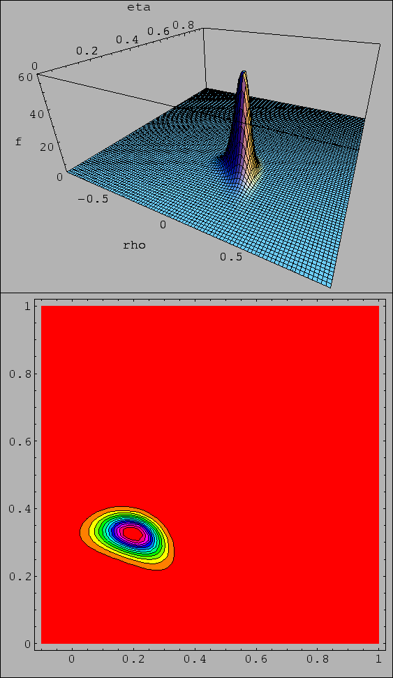
With this third reweighting, the resulting p.d.f. looses finally sign ambiguities, and becomes rather narrow, with respect to the initial space of possibilities. The 3-D plot is shown in Fig. 6.

Figure: Probability density function and contour plot 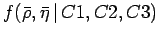$f(\bar {\rho}, \bar{\eta}\,\vert\,C1,C2,C3)$ obtained by the constraint given by $\left \vert \frac{V_{ub}}{V_{cb}} \right \vert$, $\bar{\eta}$ and $\Delta m_d$ (see remarks in text and in caption of Fig. 1 about the interpretation of the contour plot).

At this point we can evaluate expected value and standard uncertainty of the quantities of interest:

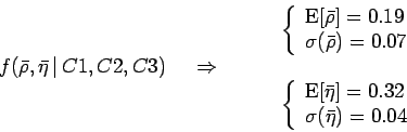$$f(\bar {\rho}, \bar{\eta}\,\vert\,C1,C2,C3)\hspace{0.5cm} \R... ...2 \\ \sigma(\bar{\eta})=0.04 \end{array}\right. \end{array}$$ (16)