Next: Conclusions
Up: Poisson background on the
Previous: Inferring
The histograms of
Fig. 11 show examples of the probability
distributions of  for
for  and three different
hypotheses for
and three different
hypotheses for  .
.
Figure:
Inference about (histograms)
and  (continuous lines)
for
(continuous lines)
for  and
and  ,
assuming and three values of
: 0.75, 0.25 and 0.95 (top down).
,
assuming and three values of
: 0.75, 0.25 and 0.95 (top down).
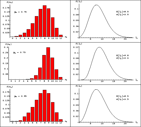 |
These distributions quantify how much we believe that
out of the observed  belong to the signal.
[By the way, the number
belong to the signal.
[By the way, the number  of background objects
present in the data can be inferred as complement
to , since the two numbers are linearly dependent. It follows
that
of background objects
present in the data can be inferred as complement
to , since the two numbers are linearly dependent. It follows
that
 .]
.]
A different question is to infer the the Poisson  of the signal. Using once more Bayes theorem we get,
under the hypothesis of signal objects:
of the signal. Using once more Bayes theorem we get,
under the hypothesis of signal objects:
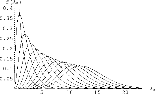
Assuming a uniform prior for we get
(see e.g. Ref. [2]):
with expected value and variance both equal to
 and mode equal to (the expected value is shifted
on the right side of the mode because the distribution is skewed
to the right).
Figure 12
shows these pdf's, for ranging from 0 to 12 and
assuming a uniform prior for .
and mode equal to (the expected value is shifted
on the right side of the mode because the distribution is skewed
to the right).
Figure 12
shows these pdf's, for ranging from 0 to 12 and
assuming a uniform prior for .
Figure:
Inference of depending on the ,
ranging from 0 to 12 (left to right curves).
 |
As far the pdf of that depends on all possible
values of , each with is probability, is concerned,
we get from probability theory
[and remembering that, indeed,
 is equal to
 , because depends only on
, and then the other way around]:
, because depends only on
, and then the other way around]:
i.e. the pdf of is the weighted
average2
of the several depending pdf's.
The results for the example we are considering in this
section are given in the plots of Fig. 11.
Next: Conclusions
Up: Poisson background on the
Previous: Inferring
Giulio D'Agostini
2004-12-13