Next: Poisson model
Up: Inferring numerical values of
Previous: Gaussian model
Binomial model
In a large class of experiments, the observations consist of counts,
that is, a number of things (events, occurrences, etc.).
In many processes of physics interests the
resulting number of counts is described probabilistically by a binomial
or a Poisson model.
For example, we want to draw an
inference about the efficiency of a detector, a branching ratio
in a particle decay or a rate from a measured number of counts
in a given interval of time.
The binomial distribution describes
the probability of randomly obtaining  events (`successes')
in
events (`successes')
in  independent trials, in each of which we assume the same probability
 that the event will happen. The probability function is
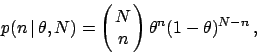 |
(37) |
where the leading factor is the well-known binomial coefficient,
namely
 .
We wish to infer from an observed number of counts in trials.
Incidentally, that was the
``problem in the doctrine of chances'' originally treated by Bayes
(1763), reproduced e.g. in (Press 1992). Assuming a uniform prior for ,
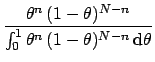
by Bayes' theorem the posterior distribution for is
proportional to the likelihood, given by Eq. (37):
.
We wish to infer from an observed number of counts in trials.
Incidentally, that was the
``problem in the doctrine of chances'' originally treated by Bayes
(1763), reproduced e.g. in (Press 1992). Assuming a uniform prior for ,
by Bayes' theorem the posterior distribution for is
proportional to the likelihood, given by Eq. (37):
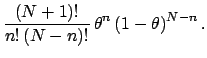
Figure 1:
Posterior probability density function of the binomial parameter
, having observed successes in trials.
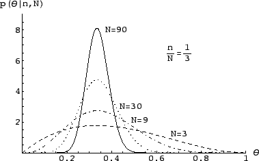 |
Some examples of this distribution for various values of and
are shown in Fig. 1.
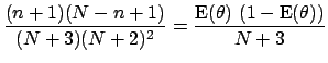
Expectation, variance, and mode of this distribution are:
where the mode has been indicated with
 .
Equation (40) is known as the Laplace formula.
For large values of and
.
Equation (40) is known as the Laplace formula.
For large values of and  the expectation of tends to
,
and
the expectation of tends to
,
and  becomes approximately Gaussian.
This result is nothing but a reflection
of the well-known asymptotic Gaussian behavior of
becomes approximately Gaussian.
This result is nothing but a reflection
of the well-known asymptotic Gaussian behavior of
 .
For large the uncertainty about
goes like
.
For large the uncertainty about
goes like  . Asymptotically, we are practically
certain that is equal to the relative frequency of that class
of events observed in the past. This is how the frequency based
evaluation of probability is promptly recovered in the Bayesian approach,
under well defined assumptions.
. Asymptotically, we are practically
certain that is equal to the relative frequency of that class
of events observed in the past. This is how the frequency based
evaluation of probability is promptly recovered in the Bayesian approach,
under well defined assumptions.
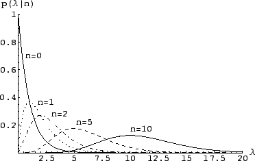
Figure 2:
The posterior distribution for the Poisson parameter  ,
when counts are observed in an experiment.
,
when counts are observed in an experiment.
 |
Next: Poisson model
Up: Inferring numerical values of
Previous: Gaussian model
Giulio D'Agostini
2003-05-13