Let us continue with the case in which we know so little about
appropriate values of the parameters
that a uniform distribution is a practical choice for the prior.
Equation (52)
becomes
The set of
![]() that is most likely is that which maximizes
that is most likely is that which maximizes
![]() , a result known as the
maximum likelihood principle. Here it has been
obtained again as a special case of a more general
framework, under
clearly stated hypotheses, without need to introduce new ad hoc rules.
Note also that the inference does not depend
on multiplicative factors in the likelihood.
This is one of the ways to state the
likelihood principle, ideally desired by frequentists,
but often violated. This `principle' always and naturally
holds in Bayesian statistics.
It is important to remark that
the use of unnecessary principles is dangerous, because there
is a tendency to use them
uncritically. For example, formulae resulting from
maximum likelihood are often used also when
non-uniform reasonable priors should be
taken into account, or when the shape of
, a result known as the
maximum likelihood principle. Here it has been
obtained again as a special case of a more general
framework, under
clearly stated hypotheses, without need to introduce new ad hoc rules.
Note also that the inference does not depend
on multiplicative factors in the likelihood.
This is one of the ways to state the
likelihood principle, ideally desired by frequentists,
but often violated. This `principle' always and naturally
holds in Bayesian statistics.
It is important to remark that
the use of unnecessary principles is dangerous, because there
is a tendency to use them
uncritically. For example, formulae resulting from
maximum likelihood are often used also when
non-uniform reasonable priors should be
taken into account, or when the shape of
![]() is far from being multi-variate Gaussian. (This is
a kind of ancillary
default hypothesis that comes together with this principle,
and is the source of the often misused `
is far from being multi-variate Gaussian. (This is
a kind of ancillary
default hypothesis that comes together with this principle,
and is the source of the often misused `
![]() ' rule
to determine probability intervals.)
' rule
to determine probability intervals.)
The usual least squares formulae are easily
derived if we take the
well-known case of pairs ![]() (the generic
(the generic
![]() stands for all data points)
whose true values are related by a deterministic function
stands for all data points)
whose true values are related by a deterministic function
![]() and
with Gaussian errors only in the ordinates, i.e.
we consider
and
with Gaussian errors only in the ordinates, i.e.
we consider
![]() .
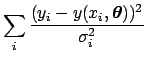
In the case of independence of the measurements, the
likelihood-dominated result becomes,
.
In the case of independence of the measurements, the
likelihood-dominated result becomes,
![$\displaystyle \prod_i \exp\left[
-\frac{(y_i-y(x_i,{\mbox{\boldmath$\theta$}}))^2}{2\,\sigma_{i}^2}\right]$](img274.png) |
(62) |
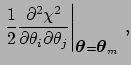
As far as the uncertainty in
![]() is concerned,
the widely-used evaluation of the covariance matrix
is concerned,
the widely-used evaluation of the covariance matrix
![]() (see Sect. 5.6)
from the Hessian,
(see Sect. 5.6)
from the Hessian,
In routine applications, the hypotheses that lead to the
maximum likelihood and least squares formulae often hold.
But when these hypotheses are not justified, we need
to characterize the result by the multi-dimensional posterior distribution
![]() , going back to the more general expression
Eq. (52).
, going back to the more general expression
Eq. (52).
The important conclusion from this section, as was the case for the definitions of probability in Sect. 3, is that Bayesian methods often lead to well-known conventional results, but without introducing them as new ad hoc rules as the need arises. The analyst acquires then a heightened sense of awareness about the range of validity of the methods. One might as well use these `recovered' methods within the Bayesian framework, with its more natural interpretation of the results. Then one can speak about the uncertainty in the model parameters and quantify it with probability values, which is the usual way in which physicists think.
![$\displaystyle \exp\left[-\frac{1}{2}\chi^2\right] \,,$](img275.png)
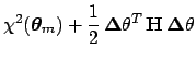
![$\displaystyle \propto \exp\left[-\frac{1}{2}
{\mbox{\boldmath$\Delta$}}\theta^T\, \mathbf{H}\,{\mbox{\boldmath$\Delta$}}\theta \right] \,,$](img289.png)
![$\displaystyle (2 \pi)^{-n/2}\, (\det\mathbf{V})^{-1/2}\,
\exp \left[-\frac{1}{2...
...Delta$}}\theta^T \,
\mathbf{V}^{-1}{\mbox{\boldmath$\Delta$}}\theta
\right] \,,$](img291.png)