Next: Inference for simple hypotheses
Up: Bayesian inference for simple
Previous: Background information
Bayes' theorem
Formally, Bayes' theorem follows from the symmetry of  expressed by Eq. (17).
In terms of
expressed by Eq. (17).
In terms of  and
and  belonging to two different
complete classes, Eq. (17) yields
belonging to two different
complete classes, Eq. (17) yields
 |
(18) |
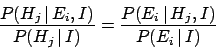
This equation says that the new condition alters
our belief in by the same updating factor by which
the condition alters our belief about .
Rearrangement yields Bayes' theorem
 |
(19) |
We have obtained a logical rule to update our beliefs on the basis of new conditions.
Note that, though Bayes' theorem is a direct consequence of the basic
rules of axiomatic probability theory, its updating power can only be fully exploited
if we can treat on the same basis expressions
concerning hypotheses and observations, causes and effects, models and data.
In most practical cases, the evaluation of  can be
quite difficult, while determining the conditional probability
can be
quite difficult, while determining the conditional probability
 might be easier. For example, think of as the probability
of observing a particular event topology in a particle physics
experiment, compared with the probability of
the same thing given a value of the hypothesized particle mass (), a given
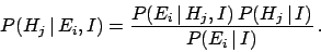
detector, background conditions, etc. Therefore, it is convenient to rewrite
in Eq. (19)
in terms of the quantities in the numerator,
using Eq. (13), to obtain
might be easier. For example, think of as the probability
of observing a particular event topology in a particle physics
experiment, compared with the probability of
the same thing given a value of the hypothesized particle mass (), a given
detector, background conditions, etc. Therefore, it is convenient to rewrite
in Eq. (19)
in terms of the quantities in the numerator,
using Eq. (13), to obtain
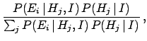
which is the better-known form of Bayes' theorem. Written this way,
it becomes evident that the denominator of the r.h.s.
of Eq. (20)
is just a normalization factor and we can focus
on just the numerator:
In words
where the posterior (or final state) stands for the probability
of , based on the
new observation , relative to the prior (or initial) probability.
(Prior probabilities are often indicated with  .)
The conditional probability
.)
The conditional probability
 is called the
likelihood. It is literally the probability of the observation
given the specific hypothesis . The term likelihood can
lead to some confusion, because it is often misunderstood to mean
``the likelihood that comes from .''
However,
this name implies to consider
a mathematical function of
for a fixed and in that framework it is usually written as
is called the
likelihood. It is literally the probability of the observation
given the specific hypothesis . The term likelihood can
lead to some confusion, because it is often misunderstood to mean
``the likelihood that comes from .''
However,
this name implies to consider
a mathematical function of
for a fixed and in that framework it is usually written as
 to emphasize the functionality.
We caution the reader that one sometimes even finds
the notation
to emphasize the functionality.
We caution the reader that one sometimes even finds
the notation
 to indicate exactly
.
to indicate exactly
.
Next: Inference for simple hypotheses
Up: Bayesian inference for simple
Previous: Background information
Giulio D'Agostini
2003-05-13