Next: Probability rules for uncertain
Up: Rules of probability
Previous: Probability of simple propositions
Probability of complete classes
These formulae become more interesting when we consider a set of
propositions  that all together form a tautology
(i.e., they are exhaustive) and are mutually exclusive.
Formally
that all together form a tautology
(i.e., they are exhaustive) and are mutually exclusive.
Formally
When these conditions apply, the set  is said to form a complete class.
The symbol
is said to form a complete class.
The symbol  has been chosen because we shall soon interpret
as a set of hypotheses.
has been chosen because we shall soon interpret
as a set of hypotheses.
The first (trivial) property
of a complete class is normalization, that is
which is just an extension of Eq. (6)
to a complete class
containing more than just a single proposition and its negation.
For the complete class , the generalizations of
Eqs. (6) and the use of
Eq. (4) yield:
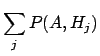
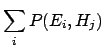
Equation (10) is the basis of what is called marginalization, which will become particularly important when
dealing with uncertain variables: the probability of  is
obtained by the summation over all possible
constituents
contained in . Hereafter, we avoid explicitly writing the
limits of the summations, meaning that they extend over all
elements of the class. The constituents are `
is
obtained by the summation over all possible
constituents
contained in . Hereafter, we avoid explicitly writing the
limits of the summations, meaning that they extend over all
elements of the class. The constituents are ` ,' which,
based on the complete class of hypotheses
,' which,
based on the complete class of hypotheses  , themselves form
a complete class, which can be easily proved.
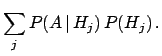
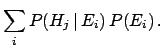
Equation (11) shows that the probability of any proposition
is given by a weighted average of all conditional probabilities,
subject to hypotheses forming a complete class, with the weight
being the probability of the hypothesis.
, themselves form
a complete class, which can be easily proved.
Equation (11) shows that the probability of any proposition
is given by a weighted average of all conditional probabilities,
subject to hypotheses forming a complete class, with the weight
being the probability of the hypothesis.
In general, there are many ways to choose complete classes
(like `bases' in geometrical spaces). Let us denote the
elements of a second complete class by  . The constituents are then
formed by the elements
. The constituents are then
formed by the elements  of the Cartesian product
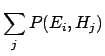
 . Equations (10) and
(11) then become the more general statements
. Equations (10) and
(11) then become the more general statements
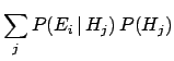
and, symmetrically,
The reason we write these formulae both ways is to
stress the symmetry of Bayesian reasoning with respect to
classes  and , though we shall soon associate them with observations (or events) and hypotheses, respectively.
Next: Probability rules for uncertain
Up: Rules of probability
Previous: Probability of simple propositions
Giulio D'Agostini
2003-05-13