Next: Conclusions
Up: From Observations to Hypotheses
Previous: Falsificationism and its statistical
Forward to the past: probabilistic reasoning
The dominant school in statistics since the beginning of last
century is based on a quite unnatural approach to probability,
in contrast to that of the founding fathers (Poisson,
Bernoulli, Bayes, Laplace, Gauss, etc.). In this approach
(frequentism) there is no room for the concept of probability
of causes,
probability of hypotheses, probability
of the values of physical quantities,
and so on.
Problems in the probability of the causes
(``the essential problem of the experimental method''![4])
have been replaced by the machinery of the hypothesis tests.
But people think naturally in terms of probability of causes,
and the mismatch between natural thinking and standard
education in statistics leads to the troubles
discussed above.
I think that the way out is simply to go back to the past.
In our time of rushed progress an invitation to
go back to century old ideas seems at least odd (imagine
a similar proposal regarding physics, chemistry or biology!).
I admit it, but I do think it is the proper way to follow.
This doesn't mean we have to drop everything done in probability and statistics
in between. Most mathematical work can be easily recovered.
In particular, we can benefit of theoretical clarifications and
progresses in probability theory of the past century.
We also take great advantage of the boost of computational capability
occurred very recently, from which both symbolic and numeric
methods have enormously benefitted.
(In fact, many frequentistic ideas had their raison d'être
in the computational barrier that the original probabilistic
approach met. Many simplified - though often
simplistic - methods were then proposed
to make the live of practitioners easier.
But nowadays computation cannot be considered any longer an excuse.)
In summary, the proposed way out can be summarized
in an invitation to use probability theory consistently.
But before you do it, you need to
review the definition of probability, otherwise it is simply
impossible to use all the power of the theory.
In the advised approach probability
quantifies how much we believe in something, i.e. we recover its
intuitive idea. Once this is done, we can
essentially use the formal probability theory based on Kolmogorov axioms
(which can indeed derived, and with a better
awareness about their meaning,
from more general principles! - but
I shall not enter this issue here).
This `new'
approach is called Bayesian because of the central
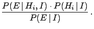
role played by Bayes theorem in learning from experimental data.
The theorem teaches how the probability of each hypothesis  has to be updated in the light of the new observation
  :
:
 stands for a background condition, or status of
information, under which the inference is made.
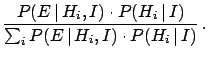
A more frequent Bayes' formula in text books, valid if the hypotheses
are exhaustive and mutually exclusive, is
stands for a background condition, or status of
information, under which the inference is made.
A more frequent Bayes' formula in text books, valid if the hypotheses
are exhaustive and mutually exclusive, is
The denominator in the right hand
side of (2)
is just a normalization factor and, as such,
it can be neglected. Moreover it is possible to
show that a similar structure holds for probability density functions
(p.d.f.) if a continuous variable is considered ( stands here
for a generic `true value', associated to a parameter of a model).
Calling `data' the overall effect ,
we get the following formulae on which inference is to be ground:
stands here
for a generic `true value', associated to a parameter of a model).
Calling `data' the overall effect ,
we get the following formulae on which inference is to be ground:
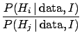
the first formula used in probabilistic comparison of hypotheses,
the second (mainly) in parametric inference.
In both cases
we have the same structure:
where `posterior' and `prior'
refer to our belief on that hypothesis, i.e.
taking or not taking into account the `data' on which the
present inference is based. The likelihood,
that is ``how much we believe
that the hypothesis
can produce the data'' (not to be confused with
``how much we believe that the data
come from the hypothesis''!), models the stochastic flow that
leads from the hypothesis to the observations, including the
best modeling of the detector response. The structure
of (5) shows us that the inference based on Bayes
theorem satisfies automatically the likelihood principle
(likelihoods that differ by constant factors lead to the
same posterior).
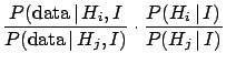
The proportionality factors in (3) and (4)
are determined by normalization, if absolute probabilities are needed.
Otherwise we can just put our attention on probability ratios:
odds are updated by data via the ratio of the
likelihoods, called Bayes factor.
There are some well known psychological (indeed
cultural and even ideological) resistances to this approach
due to the presence of the priors in the theory.
Some remarks are therefore in order:
- priors are unscapable, if we are interested in
`probabilities of causes' (stated differently,
there is no other way to relate consistently
probabilities of causes
to probabilities of effects avoiding Bayes theorem);
- therefore, you should mistrust methods that
pretend to provide `levels of confidence'
(in the sense of how much you are confident)
independently from priors (arbitrariness is often sold for objectivity!);
- in many `routine' applications the results
of measurements depend weakly on priors and
many standard formulae, usually derived from
maximum likelihood or least square principles, can be promptly
recovered
under well defined conditions of validity,
- but in other cases priors might have a strong
influence on the conclusions;
- if we understand the role and the relevance of the priors, we
shall be able to provide useful results in
the different cases (for example, when the priors
dominate the conclusions and there is no agreement
about prior knowledge, it is better
to refrain from providing probabilistic results:
Bayes factors may be considered a convenient way to
report how the experimental data push toward either
hypothesis; similarly,
upper/lower ``xx% C.L.'s'' are highly misleading and
should be simply replaced by sensitivity bounds[1]).
To make some numerical examples, let us solve two of the
problems met above.
(In order to simplify the notation the
background condition `' is not indicated explicitly
in the following formulae).
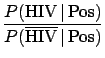
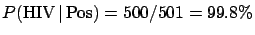
- Solution of the AIDS problem (Example 4)
-
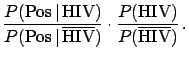
Applying Eq. (6) we get
The Bayes factor
 is equal to 1/0.002 = 500. This is
how much the information provided by the data `pushes'
towards the hypothesis `infected' with respect to
the hypothesis `healthy'. If the ratio of priors
were equal to 1 [i.e.
is equal to 1/0.002 = 500. This is
how much the information provided by the data `pushes'
towards the hypothesis `infected' with respect to
the hypothesis `healthy'. If the ratio of priors
were equal to 1 [i.e.
 !],
we would get final odds of 500, i.e.
!],
we would get final odds of 500, i.e.
 . But, fortunately,
for a randomly chosen Italian
. But, fortunately,
for a randomly chosen Italian  is not 50%.
Putting some more
reasonable numbers, that might be 1/600 or 1/700,
we have final odds of 0.83 or 0.71, corresponding
to a
is not 50%.
Putting some more
reasonable numbers, that might be 1/600 or 1/700,
we have final odds of 0.83 or 0.71, corresponding
to a
 of 45% or 42%. We understand
now the source of the mistake done by quite some people in front
of this problem: priors were unreasonable!
This is a typical situation: using the Bayesian reasoning
it is possible to show the hidden assumptions of
non-Bayesian reasonings, though most users of the latter
methods object, insisting in claiming they ``do not use priors''.
of 45% or 42%. We understand
now the source of the mistake done by quite some people in front
of this problem: priors were unreasonable!
This is a typical situation: using the Bayesian reasoning
it is possible to show the hidden assumptions of
non-Bayesian reasonings, though most users of the latter
methods object, insisting in claiming they ``do not use priors''.
- Solution of the three hypothesis problem (Example 1)
-
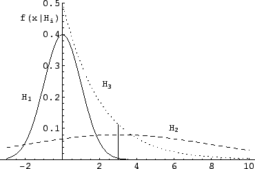
Figure 4:
Example 1: likelihoods for the three different hypotheses.
The vertical bar corresponds to the observation  .
.
 |
The Bayes factors between hypotheses  and
and  , i.e.
 , are
, are
 ,
,  and
and  .
The observation favors models 2 and 3, but the
resulting probabilities depend on priors. Assuming
prior equiprobability among the three generators we get the
following posterior probabilities for the three models:
2.3%, 41% and 57%. (In alternative,
we could know that the extraction mechanism does not
choose the three generators at random with the same probability,
and the result would change.)
.
The observation favors models 2 and 3, but the
resulting probabilities depend on priors. Assuming
prior equiprobability among the three generators we get the
following posterior probabilities for the three models:
2.3%, 41% and 57%. (In alternative,
we could know that the extraction mechanism does not
choose the three generators at random with the same probability,
and the result would change.)
Instead, if we made an analysis based on p-value we would get
that  is ``excluded'' at a 99.87% C.L. or at 99.7% C.L.,
depending whether a one-tail or a two-tail test is done.
Essentially, the perception that could be the correct cause
of is about 10-20 times smaller than that given by
the Bayesian analysis. As far as the comparison between
is ``excluded'' at a 99.87% C.L. or at 99.7% C.L.,
depending whether a one-tail or a two-tail test is done.
Essentially, the perception that could be the correct cause
of is about 10-20 times smaller than that given by
the Bayesian analysis. As far as the comparison between
 and
and  is concerned,
the p-value analysis is in practice inapplicable
(what would you do?)
and one says that both models describe about
equally well the result, which is more or less what we
get out of the Bayesian analysis. However, the latter
analysis gives some quantitative information: a slight hint
in favor of , that could be properly combined
with many other small hints coming from other pieces of
experimental information, and that, all together,
might allow us to finally arrive
to select one of the models.
is concerned,
the p-value analysis is in practice inapplicable
(what would you do?)
and one says that both models describe about
equally well the result, which is more or less what we
get out of the Bayesian analysis. However, the latter
analysis gives some quantitative information: a slight hint
in favor of , that could be properly combined
with many other small hints coming from other pieces of
experimental information, and that, all together,
might allow us to finally arrive
to select one of the models.
Next: Conclusions
Up: From Observations to Hypotheses
Previous: Falsificationism and its statistical
Giulio D'Agostini
2004-12-22