


Next: Frequentistic coverage
Up: Appendix on probability and
Previous: Are the beliefs in
Contents
Biased Bayesian estimators
and Monte Carlo checks of
Bayesian procedures
This problem has already been raised in Sections
![[*]](file:/usr/lib/latex2html/icons/crossref.png) and . We have seen there
that the expected value of a parameter can be considered, somehow,
to be analogous to the estimators8.10 of the frequentistic approach.
It is well known, from courses on conventional statistics, that
one of the nice properties an estimator should have is that
of being free of bias.
and . We have seen there
that the expected value of a parameter can be considered, somehow,
to be analogous to the estimators8.10 of the frequentistic approach.
It is well known, from courses on conventional statistics, that
one of the nice properties an estimator should have is that
of being free of bias.
Let us consider the case of Poisson and binomial distributed
observations, exactly as they have been treated in
Sections and , i.e. assuming a
uniform prior.
Using the typical notation of frequentistic analysis, let us
indicate with  the parameter to be inferred,
with
the parameter to be inferred,
with
 its estimator.
- Poisson:
-
 ;
;  indicates the possible observation
and
is the estimator in the light of :
indicates the possible observation
and
is the estimator in the light of :
The estimator is biased, but consistent
(the bias become negligible when is large).
- Binomial:
-
 ; after
  trials one may observe
favourable results, and the estimator of
trials one may observe
favourable results, and the estimator of  is then
In this case as well the estimator is biased, but consistent.
What does it mean? The result looks worrying at first sight,
but, in reality, it is the analysis of bias that is misleading.
In fact:
- the initial intent is to reconstruct at best
the parameter, i.e. the true value of the physical quantity
identified with it;
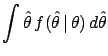
- the freedom from bias requires only that
the expected value of the estimator
should equal the value of the
parameter,
for a given value of the parameter,
But what is the true value of ? We don't know, otherwise
we would not be wasting our time trying to estimate it
(always keep real situations in mind!).
For this reason, our considerations
cannot depend only on the fluctuations of
around
, but also on the different degrees of belief of the possible
values of .
Therefore they must depend also on
 .
For this reason, the Bayesian result is that which makes the
best use8.11 of the state of knowledge about
and of the distribution of
for each possible value .
This can be easily understood by going back to the examples of
Section .
It is also easy to see that the freedom from bias
of the frequentistic approach requires
to
be uniformly distributed from
.
For this reason, the Bayesian result is that which makes the
best use8.11 of the state of knowledge about
and of the distribution of
for each possible value .
This can be easily understood by going back to the examples of
Section .
It is also easy to see that the freedom from bias
of the frequentistic approach requires
to
be uniformly distributed from  to
to  (implicitly, as frequentists refuse
the very concept of probability of ). Essentially,
whenever a parameter has a limited range, the frequentistic analysis
decrees that Bayesian estimators are biased.
(implicitly, as frequentists refuse
the very concept of probability of ). Essentially,
whenever a parameter has a limited range, the frequentistic analysis
decrees that Bayesian estimators are biased.
There is another important and subtle point related to this problem,
namely that of the
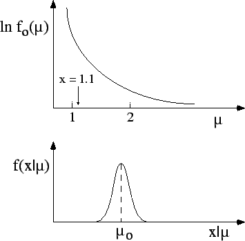
Monte Carlo check of Bayesian methods. Let us consider the case
depicted in Fig. and imagine
making a simulation, choosing the value
 ,
generating many (e.g. 10
,
generating many (e.g. 10  000) events, and considering
three different analyses:
000) events, and considering
three different analyses:
- a maximum likelihood analysis;
- a Bayesian analysis, using a flat distribution for
 ;
;
- a Bayesian analysis, using a distribution of `of the
kind'
 of Fig. ,
assuming that we have a good idea of the kind of physics
we are doing.
of Fig. ,
assuming that we have a good idea of the kind of physics
we are doing.
Which analysis will reconstruct a value closest to  ?
You don't really need to run the Monte Carlo to realize that
the first two procedures will perform equally well, while
the third one, advertised as the best in these notes, will
systematically underestimate !
?
You don't really need to run the Monte Carlo to realize that
the first two procedures will perform equally well, while
the third one, advertised as the best in these notes, will
systematically underestimate !
Now, let us assume we have observed a value of  , for example
  .
Which analysis would you use to infer the value of ?
Considering only the results of the
Monte Carlo simulation it seems obvious
that one should choose one of the first two, but
certainly not the third!
.
Which analysis would you use to infer the value of ?
Considering only the results of the
Monte Carlo simulation it seems obvious
that one should choose one of the first two, but
certainly not the third!
This way of thinking is wrong, but unfortunately
it is often used by practitioners who have no time to understand
what is behind Bayesian reasoning, who perform some Monte Carlo tests,
and decide that the Bayesian theorem does not
work!8.12 The solution
to this apparent paradox is simple.
If you
believe that is distributed like
of Fig. , then you should use this
distribution in the analysis and also
in the generator. Making a simulation
based only on a single true value, or on a set of
points with equal weight, is equivalent to assuming
a flat distribution for and, therefore,
it is not surprising
that the most grounded Bayesian analysis is that
which performs worst
in the simple-minded frequentistic checks.
It is also worth remembering that priors are not
just mathematical objects to be plugged into Bayes' theorem,
but must reflect prior knowledge. Any inconsistent
use of them leads to paradoxical results.
Next: Frequentistic coverage
Up: Appendix on probability and
Previous: Are the beliefs in
Contents
Giulio D'Agostini
2003-05-15
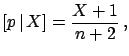
![$\displaystyle [p\,\vert\,X] = \frac{X+1}{n+2} \,,$](img1203.png)
 i.e.
i.e.