Naïve procedure

We have learned that we can infer

$$f(\lambda\,\vert\,x=0) = e^{-\lambda}$$

and, from the relation $\lambda = k\,(1-m^2/E_b^2)^{3/2}$ we get

$$f(m) = 3\,k\,\frac{m}{E_b^2}\left(1-\frac{m^2}{E_b^2}\right)^{\frac{1}{2}} \exp{\left[-k\,\left(1-\frac{m^2}{E_b^2}\right)^{\frac{3}{2}}\right]}\,,$$ (9.17)

which is clearly wrong, since it goes to 0 for $m\rightarrow E_b$. Figure shows the plot of $f(m)$, obtained with the following Mathematica code:

(********************************************************)
ClearAll["Global`*"]

(* Experiment A has been run at beam energy 0.09, with 
sensitivity factor k=20, threshold function beta^3,
and has observed 0 events.*)    

ka=20
eba=0.09

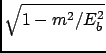
v=Sqrt[1-(m/eba)^2]
lambda= ka*v^3

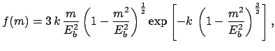
(* f(m) obtained from f(lambda)=Exp[-lambda] by lambda=k beta^3
   (threshold factor) using p.d.f transformation *)

fl=Exp[-lambda]
J=Abs[D[lambda, m]]
fm=fl*J

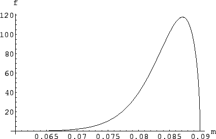
(* check normalization and plot *)

NIntegrate[fm, {m, 0, eba}]
Plot[fm, {m, 0.06, eba}, AxesLabel -> {m, f}]

(* Strange result: try to figure out the reason! *)
(********************************************************)

Figure: Inference on the mass of the hypothetical particle $H$ with the information of experiment $A$, obtained from the intermediate inference on $\lambda$ assuming a uniform prior on this quantity. The result looks very strange.

The result is against our initial rational belief and we refuse to accept it. The origin of this strange behaviour is due to the term $\sqrt{1-m^2/E_b^2}$ in () that comes directly from the Jacobian of the transformation and, indirectly from having assumed a prior uniform in $\lambda$. To solve the problem we have to change prior. But this seems to be cheating. Should not the prior come before? How can we change it after we have seen the final distribution?

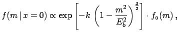
We should not confuse what we think with how we model it. The intuitive prior is on the mass values, and this prior should be flat (at least at this stage of the analysis, as discussed in Section ). Unfortunately, what is flat in $\lambda$ is not flat in $m$, and vice versa. This problem has been discussed in Section . In fact, it is not really a problem of probability, but of extrapolating intuitive probability (which is at the basis of subjective probability and only deals with discrete numbers) to continuous variables. This is the price we pay for using all the mathematical tools of differential calculus. But one has to be very careful in formulating the problem. If one wants to get rid of these problems, one may discretize $\lambda$ and $m$ in a way which is consistent with to the experimental resolution. If we discretize, a flat distribution in $m$ is mapped to a flat distribution in $\lambda$. And the problems caused by the Jacobian go away with the Jacobian itself, at the expense of some complications in computation.