Correct procedure

In order to solve the problem consistently with our beliefs, we have to avoid the intermediate inference^9.5 on $\lambda$, and write prior and likelihood directly in terms of $m$:

$$f(m\,\vert\,x=0) \propto \exp{\left[-k\,\left(1-\frac{m^2}{E_b^2}\right)^{\frac{3}{2}}\right]} \cdot f_\circ(m)\,,$$ (9.18)

with $f_\circ(m)=$   constant. Let us do it again with Mathematica:

(********************************************************)
(* Now let's do it right: *)

lik=Exp[-lambda]
norm=NIntegrate[lik, {m, 0, eba}]

(* fa(m) is the final distribution from experiment A, 
   under the condition that m < eba *)

fa=lik/norm
Plot[fa, {m, 0.06, eba}, AxesLabel -> {m, f}]
(********************************************************)

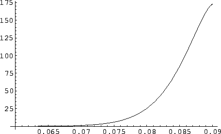
Figure: Inference on $m$ obtained from a direct inference on $m$, starting from a uniform prior in this quantity.

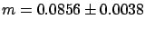
The final distribution is shown in Fig. . It is now reasonable and consistent with the expectations: The values of mass which are less believable are those which could have been produced easier, given the kinematics. From $f(m\,\vert\,x=0)$ we can calculate several results, for example a 95% upper limit, the average and the standard deviation:

(********************************************************)
NIntegrate[fa, {m, 0, 0.0782}]
ava = NIntegrate[m*fa, {m, 0, eba}]
stda = Sqrt[NIntegrate[m*fa, {m, 0, eba}] - ava^2]
(********************************************************)

We get:

$$m > 0.0782\$$ (9.19)

$$(m) = 0.0856$$ (9.20)

$$\sigma(m) = 0.0038\,.$$ (9.21)