


Next: Systematic errors
Up: Evaluation of uncertainty: general
Previous: Direct measurement in the
Contents
The case of quantities measured indirectly
is conceptually very easy, as there is
nothing to `think'. Since all values of the quantities
are associated with random numbers,
the uncertainty on the
input quantities is propagated to that of
output quantities, making use of the rules
of probability. Calling  ,
,  and
and
 the generic quantities, the inferential scheme is:
![\begin{displaymath}\begin{array}{l} f(\mu_1\,\vert\,{data}_1) \\ f(\mu_2\,\vert\...
...[\mu_3=g(\mu_1,\mu_2)] {} f(\mu_3\,\vert\,{data}_1,{data}_2)\,.\end{displaymath}](img159.png) |
(2.4) |
The problem of going from the probability density
functions (p.d.f.'s) of
and
to that of makes use of probability calculus, which can
become difficult, or impossible to do analytically,
if p.d.f.'s or
 are complicated mathematical functions. Anyhow, it is interesting to
note that the solution to the problem is, indeed, simple, at least
in principle. In fact,
are complicated mathematical functions. Anyhow, it is interesting to
note that the solution to the problem is, indeed, simple, at least
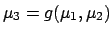
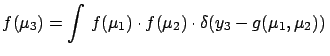
in principle. In fact,  is given, in the most general case,
by
is given, in the most general case,
by
where  is the Dirac delta function. The formula
can be easily extended to many variables, or even correlations
can be taken into account (one needs only to replace the product of
individual p.d.f.'s
by a joint p.d.f.).
Equation (
is the Dirac delta function. The formula
can be easily extended to many variables, or even correlations
can be taken into account (one needs only to replace the product of
individual p.d.f.'s
by a joint p.d.f.).
Equation (![[*]](file:/usr/lib/latex2html/icons/crossref.png) ) has a simple intuitive
interpretation: the infinitesimal
probability element
) has a simple intuitive
interpretation: the infinitesimal
probability element
 depends on `how many'
(we are dealing with infinities!) elements
depends on `how many'
(we are dealing with infinities!) elements
 contribute to it, each weighed with the p.d.f. calculated in the point
 . An alternative
interpretation of Eq. (), very useful in
applications, is to think of a Monte Carlo simulation,
where all possible values of and enter with
their distributions, and correlations are properly
taken into account. The histogram of calculated from
. An alternative
interpretation of Eq. (), very useful in
applications, is to think of a Monte Carlo simulation,
where all possible values of and enter with
their distributions, and correlations are properly
taken into account. The histogram of calculated from
 will `tend' to for a large
number of generated
events.2.16
will `tend' to for a large
number of generated
events.2.16
In routine cases the propagation is done in an approximate way,
assuming linearization of
and normal distribution
of . Therefore only
variances and covariances need to be calculated.
The well-known error propagation formulae are
recovered (Section ),
but now with a well-defined probabilistic meaning.
Next: Systematic errors
Up: Evaluation of uncertainty: general
Previous: Direct measurement in the
Contents
Giulio D'Agostini
2003-05-15
 d
d