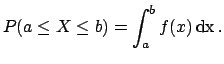
Continuous variables: probability and density function

Moving from discrete to continuous variables there are the usual problems with infinite possibilities, similar to those found in Zeno's ``Achilles and the tortoise'' paradox. In both cases the answer is given by infinitesimal calculus. But some comments are needed:

• The probability of each of the realizations of $X$ is zero ($P(X=x)=0$); but this does not mean that each value is impossible, otherwise it would be impossible to get any result.
• Although all values $x$ have zero probability, one usually assigns different degrees of belief to them, quantified by the probability density function $f(x)$. Writing $f(x_1) > f(x_2)$, for example, indicates that our degree of belief in $x_1$ is greater than that in $x_2$.
• The probability that a random variable lies inside a finite interval, for example $P(a\leq X \leq b)$, is instead finite. If the distance between $a$ and $b$ becomes infinitesimal, then the probability becomes infinitesimal too. If all the values of $X$ have the same degree of belief (and not only equal numerical probability $P(x)=0$) the infinitesimal probability is simply proportional to the infinitesimal interval $\rm {d}P=k\,\rm {d}x$. In the general case the ratio between two infinitesimal probabilities around two different points will be equal to the ratio of the degrees of belief in the points (this argument implies the continuity of $f(x)$ on either side of the values). It follows that $\rm {d}P=f(x)\,\rm {d}x$ and then

  $$P(a \leq X \leq b)= \int_{a}^{b}f(x)\, \rm {d} x\, .$$ (4.25)

  
  

• $f(x)$ has a dimension inverse to that of the random variable.

After this short introduction, here is a list of definitions, properties and notations:

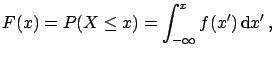
Cumulative distribution function:

$$F(x) = P(X \leq x) = \int_{-\infty}^{x} f(x^\prime) \, \mathrm{d} x^\prime \, ,$$ (4.26)

or

$$f(x) = \frac{\rm {d}F(x)}{\rm {d}x}$$ (4.27)

Properties of $f(x)$ and $F(x)$:

• $f(x) \geq 0\,\,$,
• $\int_{-\infty}^{+\infty} f(x)\,\rm {d}x=1\,\,$,
• $0\leq F(x)\leq 1$,
• $P(a\leq X \leq b) = \int_a^bf(x)\,\rm {d}x = \int_{-\infty}^b f(x)\,\rm {d}x -\int_{-\infty}^af(x)\,\rm {d}x = F(b)-F(a)$,
• if $x_2 > x_1$ then $F(x_2) \ge F(x_1)$,
• $\lim_{x\rightarrow -\infty} F(x) = 0$,
  $\lim_{x\rightarrow +\infty} F(x) = 1$.

Expectation value:

$$[X] = \int_{-\infty}^{+\infty}x\, f(x)\,\rm {d}x,$$ (4.28)

$$[g(X)] = \int_{-\infty}^{+\infty}g(x)\, f(x)\,\rm {d}x.$$ (4.29)

Uniform distribution:

^4.1

$X \sim {\cal K}(a,b)$:

$$f(x\,\vert\,{\cal K}(a,b)) = \frac{1}{b-a} \hspace{0.6cm}(a\le x \le b),$$ (4.30)

$$F(x\,\vert\,{\cal K}(a,b)) = \frac{x-a}{b-a}\, .$$ (4.31)

Expectation value and standard deviation:

$$\mu = \frac{a+b}{2},$$ (4.32)

$$\sigma = \frac{b-a}{\sqrt{12}}\,.$$ (4.33)

Normal (Gaussian) distribution:

$X\sim {\cal N}(\mu,\sigma)$:

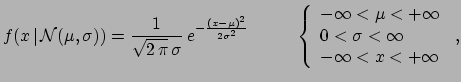$$f(x\,\vert\,{\cal N}(\mu,\sigma)) =\frac{1}{\sqrt{2\,\pi}\,\sigma... ...u < +\infty\\ 0 < \sigma < \infty\\ -\infty < x < +\infty \end{array}\right.\,,$$ (4.34)

where $\mu$ and $\sigma$ (both real) are the expectation value and standard deviation^4.2, respectively.

Standard normal distribution:

the particular normal distribution of mean 0 and standard deviation 1, usually indicated by $Z$:

$$Z\sim {\cal N}(0,1)\,.$$ (4.35)

Exponential distribution:

$T \sim {\cal E}(\tau)$:

$$f(t\,\vert\,{\cal E}(\tau)) = \frac{1}{\tau}\, e^{-t/\tau} \hspace{1.3 cm} \left\{ \begin{array}{c} 0 \le \tau < \infty, \\ 0 \le t < \infty \end{array}\right.$$ (4.36)

$$F(t\,\vert\,{\cal E}(\tau)) = 1-e^{-t/\tau}.$$ (4.37)

We use the symbol $t$ instead of $x$ because this distribution will be applied to the time domain.
Survival probability:

$$P(T>t) = 1- F(t\,\vert\,{\cal E}(\tau)) = e^{-t/\tau}.$$ (4.38)

Expectation value and standard deviation:

$$\mu = \tau$$ (4.39)

$$\sigma = \tau.$$ (4.40)

The real parameter $\tau$ has the physical meaning of lifetime.

Poisson $\leftrightarrow$ Exponential:

If $X$ (= ``number of counts during the time $\Delta t$'') is Poisson distributed then $T$ (= ``interval of time to wait -- starting from any instant -- before the first count is recorded'') is exponentially distributed:

$$X \sim f(x\,\vert\,{\cal P}_\lambda) \Longleftrightarrow T \sim f(x\,\vert\,{\cal E}(\tau))$$ (4.41)

$$(\tau = \frac{\Delta T}{\lambda}) .$$ (4.42)