Next: Central limit theorem
Up: Random variables
Previous: Continuous variables: probability and
Contents
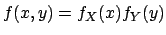
We only consider the case of two continuous variables ( and
and  ).
The extension to more variables is straightforward.
The infinitesimal element of probability is
).
The extension to more variables is straightforward.
The infinitesimal element of probability is
 , and the probability
density function
, and the probability
density function
 |
(4.43) |
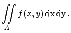
The probability of finding the variable inside a certain
area  is
is
 |
(4.44) |
- Marginal distributions:
-
The subscripts and indicate that
 and
and  are only functions of
and , respectively (to avoid fooling around with different
symbols to indicate the generic function), but in most cases
we will drop the subscripts if the context helps in resolving
ambiguities.
are only functions of
and , respectively (to avoid fooling around with different
symbols to indicate the generic function), but in most cases
we will drop the subscripts if the context helps in resolving
ambiguities.
- Conditional distributions:
-
 |
 |
 |
(4.47) |
 |
|
 |
(4.48) |
 |
|
 |
(4.49) |
| |
|
 |
(4.50) |
- Independent random variables
-
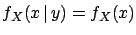 |
(4.51) |
(it implies
 and
and
 .)
.)
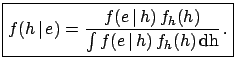
- Bayes' theorem for continuous random variables
-
 |
(4.52) |
(Note added: see proof in section ![[*]](file:/usr/lib/latex2html/icons/crossref.png) .)
.)
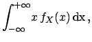
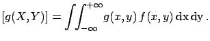
- Expectation value:
-
and analogously for . In general
E![$\displaystyle [g(X,Y)] = \int\!\!\int_{-\infty}^{+\infty} \!g(x,y)\, f(x,y)\, \rm {d}x\,\rm {d}y\,.$](img507.png) |
(4.55) |
- Variance:
-
and analogously for .
- Covariance:
-
If and are independent, then
E![$ [XY]=$](img516.png) E
E![$ [X]\cdot$](img517.png) E
E![$ [Y]$](img518.png) and hence
Cov
and hence
Cov (the opposite is true only if ,
 ).
).
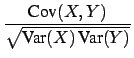
- Correlation coefficient:
-
- Linear combinations of random variables:
-
If
 , with
  real, then:
 E E![$\displaystyle [Y]$](img528.png) |
|
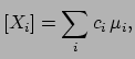 E E![$\displaystyle [X_i] = \sum_ic_i\,\mu_i,$](img530.png) |
(4.61) |
 Var Var |
|
 Var Var Cov Cov |
(4.62) |
| |
|
Var Cov Cov |
(4.63) |
| |
|
 |
(4.64) |
| |
|
 |
(4.65) |
| |
|
 |
(4.66) |
 has been written in different ways, with
increasing levels of compactness, that can be found
in the literature. In particular, () and
() use the notations
has been written in different ways, with
increasing levels of compactness, that can be found
in the literature. In particular, () and
() use the notations
 Cov
Cov and
and
 , and the fact that,
by definition,
, and the fact that,
by definition,
 .
.
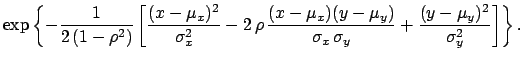
- Bivariate normal distribution:
-
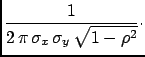
Joint probability density function
of and with correlation coefficient 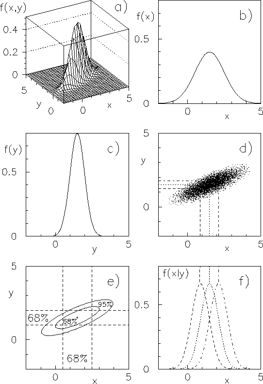 (see Fig. ):
Figure:
Example of bivariate normal distribution.
 |
Marginal distributions:
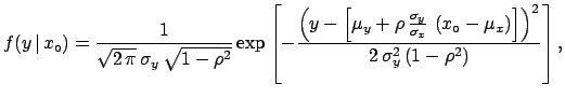
Conditional distribution:
![$\displaystyle f(y\,\vert\,x_\circ) = \frac{1}{\sqrt{2\,\pi}\,\sigma_y\,\sqrt{1-...
...(x_\circ-\mu_x\right)\right] \right)^2} {2\,\sigma_y^2\,(1-\rho^2)} \right]}\,,$](img554.png) |
(4.70) |
i.e.
 |
(4.71) |
The condition  squeezes the standard deviation and shifts
the mean of .
squeezes the standard deviation and shifts
the mean of .
Next: Central limit theorem
Up: Random variables
Previous: Continuous variables: probability and
Contents
Giulio D'Agostini
2003-05-15
 E
E![$\displaystyle [X]$](img452.png)