


Next: Distribution of a sample
Up: Central limit theorem
Previous: Central limit theorem
Contents
The well-known central limit theorem plays
a crucial role in statistics
and justifies the enormous importance
that the normal distribution has in many practical applications
(this is why it appears on 10 DM notes).
We have reminded ourselves in (![[*]](file:/usr/lib/latex2html/icons/crossref.png) )-()
of the expression of the mean and variance of a linear combination
of random variables,
)-()
of the expression of the mean and variance of a linear combination
of random variables,
in the most general case, which includes
correlated variables (
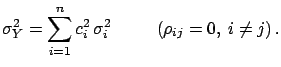 ). In the case of
independent variables the variance is
given by the simpler, and better known,
expression
). In the case of
independent variables the variance is
given by the simpler, and better known,
expression
 |
(4.72) |
This is a very general statement, valid for any
number and kind of variables
(with the obvious clause that all  must be finite), but
it does not give any information about the probability distribution
of
must be finite), but
it does not give any information about the probability distribution
of  . Even if all
 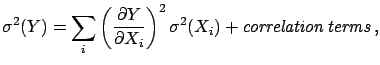 follow the same distributions
  ,
,
 is different from , with some exceptions,
one of these being the normal.
is different from , with some exceptions,
one of these being the normal.
The central limit theorem states that
the distribution of a linear combination
will be approximately normal if the variables
are independent and
 is much larger than any
single component
is much larger than any
single component
 from a non-normally distributed
. The last condition is just to guarantee that there is
no single random variable which dominates the fluctuations.
The accuracy of the approximation improves as the number of
variables
from a non-normally distributed
. The last condition is just to guarantee that there is
no single random variable which dominates the fluctuations.
The accuracy of the approximation improves as the number of
variables  increases (the theorem says ``when
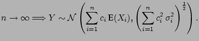 ''):
''):
 |
(4.73) |
The proof of the theorem
can be found in standard textbooks.
For practical purposes, and if one is not very interested
in the detailed behaviour of the tails, equal to 2 or 3
may already give a satisfactory approximation, especially
if the exhibits a Gaussian-like shape.
Figure:
Central limit theorem at work: The sum of
variables, for two different distributions, is shown. The values
of (top bottom) are 1, 2, 3, 5, 10, 20, 50.
 |
See for example,
Fig. , where samples of 10  000 events have
been simulated, starting from a uniform distribution and from a
crazy square-wave distribution. The latter, depicting
a kind of ``worst practical case'', shows that, already
for
000 events have
been simulated, starting from a uniform distribution and from a
crazy square-wave distribution. The latter, depicting
a kind of ``worst practical case'', shows that, already
for  the distribution of the sum is practically normal.
In the case of the uniform distribution
the distribution of the sum is practically normal.
In the case of the uniform distribution  already
gives an acceptable approximation as far as probability intervals of
one or two standard deviations
from the mean value are concerned. The figure also shows
that, starting from a triangular distribution (obtained
in the example from the sum of two uniform distributed variables),
already
gives an acceptable approximation as far as probability intervals of
one or two standard deviations
from the mean value are concerned. The figure also shows
that, starting from a triangular distribution (obtained
in the example from the sum of two uniform distributed variables),
 is already sufficient (The sum of two triangular distributed
variables is equivalent to the sum of four
uniform distributed variables.)
is already sufficient (The sum of two triangular distributed
variables is equivalent to the sum of four
uniform distributed variables.)
Next: Distribution of a sample
Up: Central limit theorem
Previous: Central limit theorem
Contents
Giulio D'Agostini
2003-05-15