Next: Measurements close to the
Up: Normally distributed observables
Previous: Final distribution, prevision and
Contents
Combination of several measurements
Let us imagine making a second set of measurements of the physical
quantity, which we assume unchanged from the previous
set of measurements. How will our knowledge of  change after
this new information? Let us call
change after
this new information? Let us call
 and
and
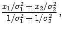
 the new average and standard
deviation of the average
(
the new average and standard
deviation of the average
(
 may be different from
  of the sample of
 measurements), respectively.
Applying
Bayes' theorem
a second time
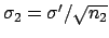
we now have to use as initial distribution
the final probability of the previous inference:
measurements), respectively.
Applying
Bayes' theorem
a second time
we now have to use as initial distribution
the final probability of the previous inference:
 |
(5.17) |
The integral is not as simple as the previous one, but still
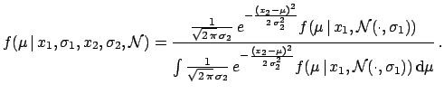
feasible analytically. The final result is
 |
(5.18) |
where
One recognizes the famous formula of the weighted
average with the inverse of the variances, usually obtained
from maximum likelihood.
There are some comments to be made.
- Bayes' theorem updates the knowledge about
in an automatic and natural way.
- If
 (and
(and  is not ``too far'' from
 ) the final result is only determined by the second
sample of measurements.
This suggests that an alternative vague a priori distribution
can be, instead of uniform, a Gaussian with a
large enough variance
and a reasonable mean.
) the final result is only determined by the second
sample of measurements.
This suggests that an alternative vague a priori distribution
can be, instead of uniform, a Gaussian with a
large enough variance
and a reasonable mean.
- The combination of the samples requires a subjective judgement
that the two samples are really coming from the same true
value . We will not discuss this point in these
notes5.3, but
a hint on how to proceed is to: take the inference on the
difference of two measurements,
 , as explained at the end of
Section
, as explained at the end of
Section ![[*]](file:/usr/lib/latex2html/icons/crossref.png) and judge yourself whether
and judge yourself whether  is
consistent with the probability density function of .
is
consistent with the probability density function of .
Next: Measurements close to the
Up: Normally distributed observables
Previous: Final distribution, prevision and
Contents
Giulio D'Agostini
2003-05-15