Next: Combination of several measurements
Up: Normally distributed observables
Previous: Normally distributed observables
Contents
Final distribution, prevision and credibility intervals of
the true value
The first application of the Bayesian inference will be that
of a normally distributed quantity. Let us take
a data sample
 of
of  measurements, of which
we calculate the average
measurements, of which
we calculate the average
 . In our formalism
is a realization of the random variable
. In our formalism
is a realization of the random variable
 . Let us assume we know the
standard deviation
. Let us assume we know the
standard deviation  of the variable
  , either
because is very large and can be estimated
accurately from the sample or because it was known a priori
(We are not going to discuss in these notes the case
of small samples and unknown variance5.2.)
, either
because is very large and can be estimated
accurately from the sample or because it was known a priori
(We are not going to discuss in these notes the case
of small samples and unknown variance5.2.) The property of the average (see Section
 ![[*]](file:/usr/lib/latex2html/icons/crossref.png) )
tells us that the
likelihood
)
tells us that the
likelihood
 is Gaussian:
 |
(5.11) |
To simplify the following notation, let us call  this average and
  the standard deviation of the average:
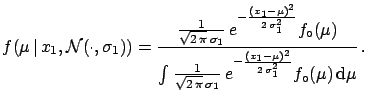
We then apply () and get
 |
(5.14) |
At this point we have to make a choice for
 . A reasonable choice
is to take, as a first guess,
a uniform distribution defined over a ``large''
interval which includes . It is not really important
how large the interval is,
for a few away
from the integrand at the denominator
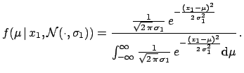
tends to zero because of the Gaussian function. What is important
is that a constant
can be simplified
in (), obtaining
. A reasonable choice
is to take, as a first guess,
a uniform distribution defined over a ``large''
interval which includes . It is not really important
how large the interval is,
for a few away
from the integrand at the denominator
tends to zero because of the Gaussian function. What is important
is that a constant
can be simplified
in (), obtaining
 |
(5.15) |
The integral in the denominator is equal to unity, since
integrating with
respect to  is equivalent to integrating with respect to .
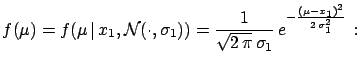
The final result is then
is equivalent to integrating with respect to .
The final result is then
 |
(5.16) |
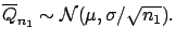
- the true value is normally distributed around ;
- its best estimate (prevision) is
E
![$ [\mu]=x_1$](img662.png) ;
;
- its variance is
 ;
;
- the ``confidence intervals'', or credibility intervals,
in which there is a certain probability of finding the
true value are easily calculable:
| Probability level |
credibility interval |
| (confidence level) |
(confidence interval) |
 |
|
| 68.3 |
|
 |
|
| 90.0 |
|
|
 |
| 95.0 |
|
|
 |
| 99.0 |
|
|
 |
| 99.73 |
|
|
 |
Next: Combination of several measurements
Up: Normally distributed observables
Previous: Normally distributed observables
Contents
Giulio D'Agostini
2003-05-15