Bayesian inference

In the Bayesian framework the inference is performed by calculating the final distribution of the random variable associated with the true values of the physical quantities from all available information. Let us call $\underline{x}=\{x_1, x_2, \ldots, x_n\}$ the n-tuple (``vector'') of observables, $\underline{\mu}=\{\mu_1, \mu_2, \ldots, \mu_n\}$ the n-tuple of the true values of the physical quantities of interest, and $\underline{h}=\{h_1, h_2, \ldots, h_n\}$ the n-tuple of all the possible realizations of the influence variables $H_i$. The term ``influence variable'' is used here with an extended meaning, to indicate not only external factors which could influence the result (temperature, atmospheric pressure, and so on) but also any possible calibration constant and any source of systematic errors. In fact the distinction between $\underline{\mu}$ and $\underline{h}$ is artificial, since they are all conditional hypotheses. We separate them simply because at the end we will ``marginalize'' the final joint distribution functions with respect to $\underline{\mu}$, integrating the joint distribution with respect to the other hypotheses considered as influence variables.

The likelihood of the sample $\underline{x}$ being produced from $\underline{h}$ and $\underline{\mu}$ and the initial probability are

$$f(\underline{x}\,\vert\,\underline{\mu}, \underline{h}, H_\circ)$$

and

$$f_\circ(\underline{\mu}, \underline{h}) = f(\underline{\mu}, \underline{h}\,\vert\, H_\circ)\,,$$ (5.1)

respectively. $H_\circ$ is intended to remind us, yet again, that likelihoods and priors -- and hence conclusions -- depend on all explicit and implicit assumptions within the problem, and in particular on the parametric functions used to model priors and likelihoods. To simplify the formulae, $H_\circ$ will no longer be written explicitly.

Using the Bayes formula for multidimensional continuous distributions [an extension of ( )] we obtain the most general formula of inference,

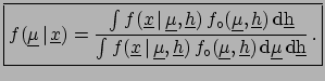$$f(\underline{\mu}, \underline{h}\,\vert\,\underline{x}) = \frac{f... ...erline{\mu}, \underline{h}) \,\rm {d}\underline{\mu}\, \rm {d}\underline{h}}\,,$$ (5.2)

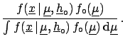
yielding the joint distribution of all conditional variables $\underline{\mu}$ and $\underline{h}$ which are responsible for the observed sample $\underline{x}$. To obtain the final distribution of $\underline{\mu}$ one has to integrate () over all possible values of $\underline{h}$, obtaining

$$\boxed{ f(\underline{\mu}\,\vert\,\underline{x}) = \frac{\int f(\... ...line{\mu}, \underline{h}) \,\rm {d}\underline{\mu}\, \rm {d}\underline{h}}\,. }$$ (5.3)

Apart from the technical problem of evaluating the integrals, if need be numerically or using Monte Carlo methods^5.1, () represents the most general form of hypothetical inductive inference. The word ``hypothetical'' reminds us of $H_\circ$.

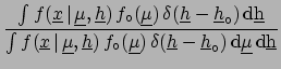
When all the sources of influence are under control, i.e. they can be assumed to take a precise value, the initial distribution can be factorized by a $f_\circ(\underline{\mu})$ and a Dirac $\delta(\underline{h}-\underline{h}_\circ)$, obtaining the much simpler formula

$$f(\underline{\mu}\,\vert\,\underline{x}) = \frac{\int f(\underline{x}\,\vert\,\underline{\mu}, \underline{h}... ...erline{h}-\underline{h}_\circ) \,\rm {d}\underline{\mu}\, \rm {d}\underline{h}}$$

$$= \frac{f(\underline{x}\,\vert\,\underline{\mu}, \underline{h}_\cir... ...}, \underline{h}_\circ) \,f_\circ(\underline{\mu})\, \rm {d}\underline{\mu}}\,.$$ (5.4)

Even if formulae ()-() look complicated because of the multidimensional integration and of the continuous nature of $\underline{\mu}$, conceptually they are identical to the example of the $\rm {d}E/\rm {d}x$ measurement discussed in Section .

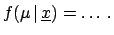
The final probability density function provides the most complete and detailed information about the unknown quantities, but sometimes (almost always $\ldots$) one is not interested in full knowledge of $f(\underline{\mu})$, but just in a few numbers which summarize at best the position and the width of the distribution (for example when publishing the result in a journal in the most compact way). The most natural quantities for this purpose are the expectation value and the variance, or the standard deviation. Then the Bayesian best estimate of a physical quantity is:

$$\widehat{\mu}_i = [\mu_i] = \int \mu_i\, f(\underline{\mu}\,\vert\,\underline{x})\, \rm {d}\underline{\mu},$$ (5.5)

$$\sigma_{\mu_i}^2\equiv (\mu_i) = [\mu_i^2] - ^2[\mu_i].$$ (5.6)

When many true values are inferred from the same data the numbers which synthesize the result are not only the expectation values and variances, but also the covariances, which give at least the correlation coefficients between the variables:

$$\rho_{ij}\equiv\rho(\mu_i,\mu_j) = \frac{\mbox{Cov}(\mu_i,\mu_j)} {\sigma_{\mu_i}\,\sigma_{\mu_j}}\,.$$ (5.7)

In the following sections we will deal in most cases with only one value to infer:

$$f(\mu\,\vert\,\underline{x}) = \ldots \,.$$ (5.8)