Next: Indirect calibration
Up: Uncertainty due to systematic
Previous: Correction for known systematic
Contents
Measuring two quantities with the same instrument
having an uncertainty of the scale offset
Let us take an example which is a little more complicated (at least from
the mathematical point of view) but conceptually very
simple and also very common in laboratory practice.
We measure two physical quantities with the same instrument,
assumed
to have an uncertainty on the ``zero'',
modelled with a normal distribution as in the
previous sections. For each of the
quantities we collect a sample of data under the same
conditions, which means that the unknown offset error does not
change from one set of measurements to the other.
Calling  and
and  the true
values,
the true
values,  and
and  the sample averages,
  and
and
 the average's standard deviations,
and
the average's standard deviations,
and  the true value of the ``zero'',
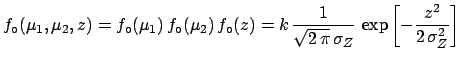
the initial probability density and the likelihood are
the true value of the ``zero'',
the initial probability density and the likelihood are
![$\displaystyle f_\circ(\mu_1,\mu_2,z)=f_\circ(\mu_1)\,f_\circ(\mu_2)\,f_\circ(z)...
...rac{1}{\sqrt{2\,\pi}\,\sigma_Z} \,\exp{\left[-\frac{z^2}{2\,\sigma_Z^2}\right]}$](img838.png) |
(5.72) |
and
respectively.
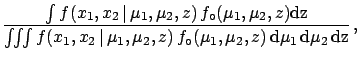
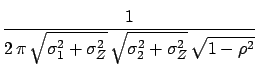
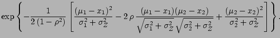
The result of the inference is now the joint probability density
function of and :
where expansion of the functions has been omitted for the
sake of clarity.
Integrating we get
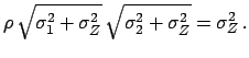
where
 |
(5.76) |
If 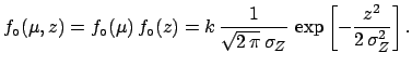 vanishes then (
![[*]](file:/usr/lib/latex2html/icons/crossref.png) ) has the simpler expression
) has the simpler expression
![$\displaystyle f(\mu_1,\mu_2) @>>{\sigma_Z\rightarrow 0}> \frac{1}{\sqrt{2\,\pi}...
...2\,\pi}\,\sigma_2} \,\exp{\left[-\frac{(\mu_2-x_2)^2}{2\,\sigma_2^2}\right]}\,,$](img848.png) |
(5.77) |
i.e. if there is no uncertainty on the offset calibration then the
joint density function
 is equal to the
product of two independent
normal functions, i.e. and
are independent.
In the general case we have to conclude the following.
is equal to the
product of two independent
normal functions, i.e. and
are independent.
In the general case we have to conclude the following.
- The effect of the common uncertainty makes the two
values correlated, since they are affected by a common
unknown
systematic error; the correlation coefficient is always non-negative
(
 ), as intuitively expected from the definition
of systematic error.
), as intuitively expected from the definition
of systematic error.
- The joint density function is a multinormal distribution
of parameters
,
 ,
,
,
,
 , and
, and 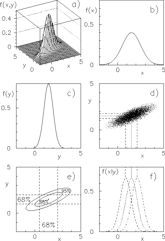 (see example of Fig. ).
- The marginal distributions are still normal:
- The covariance between and is
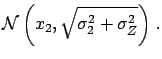
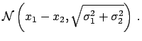
- The distribution of any function
 can be calculated
using the standard methods of probability theory. For example,
one can demonstrate that the sum
can be calculated
using the standard methods of probability theory. For example,
one can demonstrate that the sum
 and the difference
 are also normally distributed (see also the
introductory discussion to the central limit theorem
and section for the calculation of averages
and standard deviations):
are also normally distributed (see also the
introductory discussion to the central limit theorem
and section for the calculation of averages
and standard deviations):
The result can be interpreted in the following way.
- The uncertainty on the difference does not depend on the
common offset uncertainty: whatever the value of the true ``zero'' is,
it cancels in differences.
- In the sum, instead, the effect of the common
uncertainty is somewhat amplified since it enters ``in phase''
in the global uncertainty of each of the quantities.
Next: Indirect calibration
Up: Uncertainty due to systematic
Previous: Correction for known systematic
Contents
Giulio D'Agostini
2003-05-15
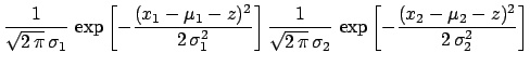
![$\displaystyle \frac{1}{\sqrt{2\,\pi}\,\sigma_1}
\,\exp{\left[-\frac{(x_1-\mu_1-...
...{2\,\pi}\,\sigma_2}
\,\exp{\left[-\frac{(x_2-\mu_2-z)^2}{2\,\sigma_2^2}\right]}$](img840.png)

![$\displaystyle \exp{
\left\{
-\frac{1}{2\,(1-\rho^2)}
\left[ \frac{(\mu_1-x_1)^2...
...sigma_Z^2}}
+\frac{(\mu_2-x_2)^2}
{\sigma_2^2+\sigma_Z^2}
\right]
\right\}
}\,.$](img846.png)