Next: Bypassing the Bayes' theorem
Up: Uncertainty due to systematic
Previous: Indirect calibration
Contents
Counting measurements in the presence of background
As an example of a different kind of systematic effect, let
us think of counting experiments in the presence of background. For
example we are searching for a new particle, we make some
selection
cuts and count  events. But we also expect
an average number of background events
events. But we also expect
an average number of background events
 ,
where
,
where  is the standard uncertainty of
 ,
not to be confused with
,
not to be confused with
 . What can we say about
 , the true value of the average number associated with the
signal? First we will treat the case in which the determination of the
expected number
of background
events is well known (
, the true value of the average number associated with the
signal? First we will treat the case in which the determination of the
expected number
of background
events is well known (
 ), and then the
general case.
), and then the
general case.
-
 :
:
- The true value of the
sum of signal and background is
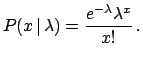 .
The likelihood is
.
The likelihood is
 |
(5.87) |
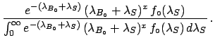
Applying Bayes' theorem we have
Choosing again
 uniform (in a reasonable interval)
this gets simplified. The integral in the denominator
can be calculated easily by parts and the final result is
uniform (in a reasonable interval)
this gets simplified. The integral in the denominator
can be calculated easily by parts and the final result is
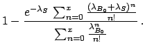
From (![[*]](file:/usr/lib/latex2html/icons/crossref.png) )-()
it is possible to calculate in the usual way the best estimate
and the
credibility intervals of .
Two particular cases are of interest:
)-()
it is possible to calculate in the usual way the best estimate
and the
credibility intervals of .
Two particular cases are of interest:
-
 :
:
- In the general case, the true value of the average
number of background events
 is unknown.
We only known that it is distributed around
with standard deviation
and probability density function
is unknown.
We only known that it is distributed around
with standard deviation
and probability density function
 ,
not necessarily a Gaussian. What changes with respect to
the previous case is the initial distribution, now a joint
function
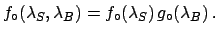
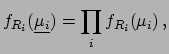
of and of . Assuming
and independent the prior density function
is
,
not necessarily a Gaussian. What changes with respect to
the previous case is the initial distribution, now a joint
function
of and of . Assuming
and independent the prior density function
is
 |
(5.92) |
We leave 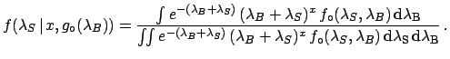 in the form of a joint distribution to
indicate that the result we shall get is the most general
for this kind of problem.
The likelihood, on the other hand, remains
the same as in the previous example.
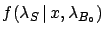
The inference of is done in the
usual way, applying Bayes' theorem and marginalizing with respect to
:
in the form of a joint distribution to
indicate that the result we shall get is the most general
for this kind of problem.
The likelihood, on the other hand, remains
the same as in the previous example.
The inference of is done in the
usual way, applying Bayes' theorem and marginalizing with respect to
:
 |
(5.93) |
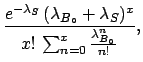
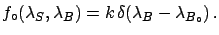
The previous case [formula ()]
is recovered if the only value allowed
for is
and
is uniform:
 |
(5.94) |
Next: Bypassing the Bayes' theorem
Up: Uncertainty due to systematic
Previous: Indirect calibration
Contents
Giulio D'Agostini
2003-05-15