Next: Normalization uncertainty
Up: Building the covariance matrix
Previous: Building the covariance matrix
Contents
Let
 be the
 results
of independent measurements
and
results
of independent measurements
and
 the (diagonal) covariance matrix.
Let us assume that they are all affected by the same calibration
constant
the (diagonal) covariance matrix.
Let us assume that they are all affected by the same calibration
constant  , having a standard uncertainty
  .
The corrected results are then
.
The corrected results are then
 .
We can assume, for
simplicity, that the most probable value of is 0, i.e.
the detector is well calibrated.
One has to
consider the calibration constant as
the physical quantity
.
We can assume, for
simplicity, that the most probable value of is 0, i.e.
the detector is well calibrated.
One has to
consider the calibration constant as
the physical quantity  , whose best estimate is
 .
A term
.
A term
 must be added to the
covariance matrix.
must be added to the
covariance matrix.
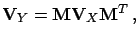
The covariance matrix of the corrected results is given by the
transformation
 |
(6.25) |
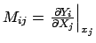
where
 .
The elements of
.
The elements of 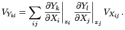 are given by
 |
(6.26) |
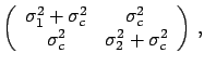
In this case we get
 |
 |
 |
(6.27) |
Cov |
|
 |
(6.28) |
 |
|
 |
(6.29) |
| |
|
 |
(6.30) |
reobtaining the results of Section ![[*]](file:/usr/lib/latex2html/icons/crossref.png) .
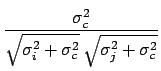
The total uncertainty on the single measurement is given by the
combination in quadrature of the individual and the common
standard uncertainties, and all the covariances are equal to
.
The total uncertainty on the single measurement is given by the
combination in quadrature of the individual and the common
standard uncertainties, and all the covariances are equal to
 .
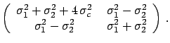
To verify, in a simple case, that the result is reasonable,
let us consider only two independent quantities
.
To verify, in a simple case, that the result is reasonable,
let us consider only two independent quantities  and
and  ,
and a calibration constant
,
and a calibration constant  , having
an expected value equal to zero. From these we can calculate
the correlated quantities
, having
an expected value equal to zero. From these we can calculate
the correlated quantities  and
and  and finally their
sum (
and finally their
sum (
 ) and difference (
 ). The results are
It follows that
as intuitively expected.
Next: Normalization uncertainty
Up: Building the covariance matrix
Previous: Building the covariance matrix
Contents
Giulio D'Agostini
2003-05-15