Appendix - Independent Gaussian errors are not a sufficient condition to rely on the standard weighted average: an instructive puzzle

Imagine we have a sample of $n$ observations, characterized by independent Gaussian errors with unkown $\mu$, associated to the true value of interest, and also unkown $\sigma$. Our main interest is to infer $\mu$, but in this case also $\sigma$ needs to be estimated from the same sample. The `estimators' (to use frequentistic vocabulary, to which most readers are most likely familiar) of $\mu$ and $\sigma$ are the aritmetic mean $\overline{x}$ and the standard deviation $s$ calculated from the sample, respectively.<sup>19</sup>In particular the `error' on $\mu$ is calculated as $s/\sqrt{n}$ (hereafter we focus on the determination of $\mu$, although a similar reasoning and a related puzzle concerns the determination of $\sigma$).

Now the question is what happens if we devide the samples in sub-samples, `determine' $\mu$ from each sub-sample and then combine the partial results. In order to avoid abstract speculations, let us concentrate on the following simulated sample:²⁰

2.691952	2.805799	3.826049	1.908438, 3.844093	2.406228	5.176920	1.925284
1.688440	2.309165	3.046256	3.211285, 2.302760	2.966700	2.301784	2.232128

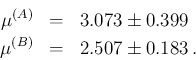
From the aritmetic average (2.7902) and the `empirical' standard deviation (0.8970), we get

$$\mu^{(All)} = 2.790 \pm 0.224$$

(the exaggerate number of decimal digits, with respect to reasonable standards, is only to make comparisons easier).

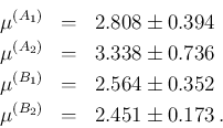
Let us now split the values into two sub-samples (first and second row, respectively). The `determinations' of $\mu$ are now

$$\begin{eqnarray*} \mu^{(A)} &=& 3.073 \pm 0.399 \\ \mu^{(B)} &=& 2.507 \pm 0.183\,. \end{eqnarray*}$$

Combining then the two results calculating the weighted average and its standard deviation, we get

$$\begin{eqnarray*} \mu^{(A\&B)} &=& 2.605 \pm 0.1660\,, \end{eqnarray*}$$

sensibly different from $\mu^{(All)}$ calculated above.

We can then split again the two samples (first four values and second four values of each row), thus getting

$$\begin{eqnarray*} \mu^{(A_1)} &=& 2.808 \pm 0.394 \\ \mu^{(A_2)} &=& 3.338 \p... ...1)} &=& 2.564 \pm 0.352 \\ \mu^{(B_2)} &=& 2.451 \pm 0.173\,. \end{eqnarray*}$$

Combining the four partial results we get then

$$\begin{eqnarray*} \mu^{(A_1\&A_2\&B_1\&B2)} &=& 2.548 \pm 0.142 \,, \end{eqnarray*}$$

different from $\mu^{(All)}$ and from $\mu^{(A\&B)}$.

What is going on? Or, more precisely, what should be the combination rule such that $\mu^{(All)}$, $\mu^{(A\&B)}$ and $\mu^{(A_1\&A_2\&B_1\&B2)}$ would be the same? (Sufficient hints are in the paper and a note could possibly follow with a detailed treatement of the case.)