Next: Conclusions Up: The Gauss' Bayes Factor Previous: Updating the probabilities of
“Now, so far as we suppose that no other data exist for the determination of the unknown quantities besides the observations,
,
etc., and, therefore, that all systems of values of these unknown quantities were equally probable previous to the observations, the probabilities, evidently, of any determinate system subsequent to the observations will be proportional to
. This is to be understood to mean that the probability that the values of the unknown quantities lie between the infinitely near limits
and
d
and
d
and
d
and
d
where the quantitywill be a constant quantity independent of
will, evidently, be the value of the integral of order
,
for each of the variablesAs we can see, it is well stated the assumption of `flat priors', as we use to say nowadays (with the original words of Gauss, in Latin: “valorum harum incognitarum ante illa observationes aeque probabilia fuisse”).13to the value
.”
It is, instead, less clear how he uses the result of his theorem (the quote at the beginning of this section follows immediately the end of the proof of the theorem, with no single word in between). The implicit intermediate step is
| (15) |
 data data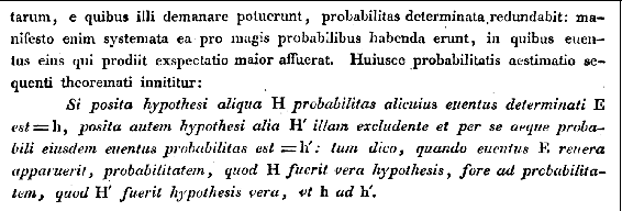 |
(16) |
|
|
||
| or |
|||
|
|
|
(17) |