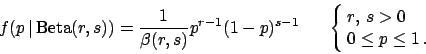
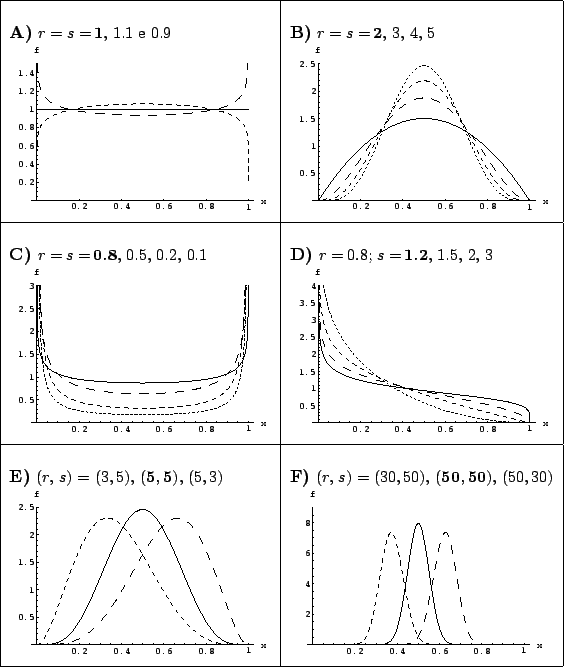
In order to see the effect of the prior, let us model it in a easy and powerful way using a beta distribution, a very flexible tool to describe many situations of prior knowledge about a variable defined in the interval between 0 and 1 (see Fig. 2).
 |
For a generic beta we get the following posterior
(neglecting the irrelevant normalization factor):
| (18) | |||
| (19) |
Expected value, mode and variance of the generic beta
of parameters ![]() and
and ![]() are:
are:
The use of the conjugate prior in this problem
demonstrates in a clear way
how the inference becomes
progressively independent from the prior information in the limit of
a large amount of data:
this happens when both ![]() and
and ![]() . In this limit we get
the same result we would get from a flat prior (
. In this limit we get
the same result we would get from a flat prior (![]() , see
Fig. 2).
For this reason in standard `routine' situation,
we can quietly and safely take a flat prior.
, see
Fig. 2).
For this reason in standard `routine' situation,
we can quietly and safely take a flat prior.
Instead, the treatment needs much more care in situations
typical of `frontier research': small numbers, and often with
no single `successes'. Let us consider the latter case and let us
assume a naïve flat prior, that it is considered to
represent `indifference' of the parameter ![]() between 0 and 1.
From Eq. (12) we get
between 0 and 1.
From Eq. (12) we get
 |
 |
(24) | ||
| (25) |
| (26) |
However, this is often not the case in frontier research.
Perhaps we were looking for a very rare process, with
a very small ![]() . Therefore, having done only 50 trials, we cannot say
to be 95% sure that
. Therefore, having done only 50 trials, we cannot say
to be 95% sure that ![]() is below 0.057. In fact, by logic, the previous
statement implies that we are 5% sure that
is below 0.057. In fact, by logic, the previous
statement implies that we are 5% sure that ![]() is above 0.057,
and this might seem too much for the scientist expert of the
phenomenology under study. (Never ask mathematicians about priors!
Ask yourselves and the colleagues you believe are the most
knowledgeable experts of what you are studying.) In general I suggest
to make the exercise of calculating a 50% upper or lower limit,
i.e. the value that divides the possible values in two equiprobable
regions: we are as confident that
is above 0.057,
and this might seem too much for the scientist expert of the
phenomenology under study. (Never ask mathematicians about priors!
Ask yourselves and the colleagues you believe are the most
knowledgeable experts of what you are studying.) In general I suggest
to make the exercise of calculating a 50% upper or lower limit,
i.e. the value that divides the possible values in two equiprobable
regions: we are as confident that ![]() is above as it is below
is above as it is below
![]() . For
. For ![]() we have
we have
![]() . If a physicist
was looking for a rare process, he/she would be highly
embarrassed to report to be 50% confident that
. If a physicist
was looking for a rare process, he/she would be highly
embarrassed to report to be 50% confident that ![]() is above 0.013.
But he/should be equally embarrassed to report to be 95% confident
that
is above 0.013.
But he/should be equally embarrassed to report to be 95% confident
that ![]() is below 0.057, because both statements are logical
consequence of the same result, that is Eq. (23).
If this is the case, a better grounded prior is needed, instead
of just a `default' uniform. For example one might thing that
several order of magnitudes in the small
is below 0.057, because both statements are logical
consequence of the same result, that is Eq. (23).
If this is the case, a better grounded prior is needed, instead
of just a `default' uniform. For example one might thing that
several order of magnitudes in the small ![]() range are considered
equally possible. This give rise to a prior that is uniform
in
range are considered
equally possible. This give rise to a prior that is uniform
in ![]() (within a range
(within a range ![]() and
and ![]() ),
equivalent to
),
equivalent to
![]() with lower and upper cut-off's.
with lower and upper cut-off's.
Anyway, instead of playing blindly with mathematics,
looking around for `objective' priors, or priors that
come from abstract arguments, it is important to understand at once
the role of prior and likelihood. Priors are logically important
to make a `probably inversion' via the Bayes formula, and
it is a matter of fact that no other route to probabilistic
inference exists. The task of the likelihood is to modify our beliefs,
distorting the pdf that models them.
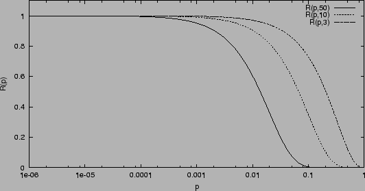
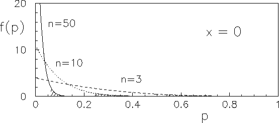
Let us plot the three
likelihoods of the three cases of Fig. 3,
rescaled to the asymptotic value
![]() (constant factors are irrelevant in likelihoods).
It is preferable to plot them in a log scale along the
abscissa to remember that several orders of magnitudes are involved
(Fig. 4).
(constant factors are irrelevant in likelihoods).
It is preferable to plot them in a log scale along the
abscissa to remember that several orders of magnitudes are involved
(Fig. 4).
We see from the figure that in the high ![]() region the beliefs
expressed by the prior are strongly dumped. If we were
convinced that
region the beliefs
expressed by the prior are strongly dumped. If we were
convinced that ![]() was in that region we have to
dramatically review our beliefs. With the increasing
number of trials, the region of `excluded' values of
was in that region we have to
dramatically review our beliefs. With the increasing
number of trials, the region of `excluded' values of ![]() increases too.
increases too.
Instead, for very small values of ![]() ,
the likelihood becomes flat, i.e. equal to the asymptotic value
,
the likelihood becomes flat, i.e. equal to the asymptotic value
![]() . The region of flat likelihood represents the values of
. The region of flat likelihood represents the values of ![]() for which the experiment loses sensitivity: if
scientific motivated priors concentrate the probability
mass in that region, then the experiment is irrelevant
to change our convictions about
for which the experiment loses sensitivity: if
scientific motivated priors concentrate the probability
mass in that region, then the experiment is irrelevant
to change our convictions about ![]() .
.
Formally the rescaled likelihood
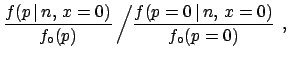 |
(28) |
We see that this ![]() function gives a way to report
an upper limit that do not depend on prior: it can be any conventional
value in the region of transition from
function gives a way to report
an upper limit that do not depend on prior: it can be any conventional
value in the region of transition from ![]() to
to
![]() . However, this limit cannot have a probabilistic
meaning, because does not depend on prior. It is instead a
sensitivity bound, roughly separating the excluded
high
. However, this limit cannot have a probabilistic
meaning, because does not depend on prior. It is instead a
sensitivity bound, roughly separating the excluded
high ![]() value from the the small
value from the the small ![]() values about which the
experiment has nothing to
say.1
values about which the
experiment has nothing to
say.1
For further discussion about the role of prior in
frontier research, applied to the Poisson process, see
Ref. [1]. For examples of experimental
results provided with the ![]() function,
see Refs. [4,5,6].
function,
see Refs. [4,5,6].