Gaussian model

Let us start with a classical example in which the response signal $d$ from a detector is described by a Gaussian error function around the true value $\mu$ with a standard deviation $\sigma$, which is assumed to be exactly known. This model is the best-known among physicists and, indeed, the Gaussian pdf is also known as normal because it is often assumed that errors are 'normally' distributed according to this function. Applying Bayes' theorem for continuous variables (see Tab. 1), from the likelihood

$$p(d\,\vert\,\mu,I) = \frac{1}{\sqrt{2\pi}\,\sigma}\exp\left[ -\frac{(d-\mu)^2}{2\,\sigma^2}\right]$$ (25)

we get for $\mu$

$$p(\mu\,\vert\,d,I) = \frac{\displaystyle\frac{1}{\sqrt{2\pi}\,\sigma}\exp\left[ -\frac... ...t[ -\frac{(d-\mu)^2}{2\,\sigma^2}\right] \,p(\mu\,\vert\,I)\,\mbox{d}\mu } \, .$$ (26)

Considering all values of $\mu$ equally likely over a very large interval, we can model the prior $p(\mu\,\vert\,I)$ with a constant, which simplifies in Eq. (26), yielding

$$p(\mu\,\vert\,d,I) = \frac{1}{\sqrt{2\pi}\,\sigma}\exp\left[ -\frac{(\mu-d)^2}{2\,\sigma^2}\right].$$ (27)

Expectation and standard deviation of the posterior distribution are $\mbox{E}(\mu)=d$ and $\sigma(\mu) = \sigma$, respectively. This particular result corresponds to what is often done intuitively in practice. But one has to pay attention to the assumed conditions under which the result is logically valid: Gaussian likelihood and uniform prior. Moreover, we can speak about the probability of true values only in the subjective sense. It is recognized that physicists, and scientists in general, are highly confused about this point (D'Agostini 1999a).

A noteworthy case of a prior for which the naive inversion gives paradoxical results is when the value of a quantity is constrained to be in the `physical region,' for example $\mu \ge 0$, while $d$ falls outside it (or it is at its edge). The simplest prior that cures the problem is a step function $\theta(\mu)$, and the result is equivalent to simply renormalizing the pdf in the physical region (this result corresponds to a `prescription' sometimes used by practitioners with a frequentist background when they encounter this kind of problem).

Another interesting case is when the prior knowledge can be modeled with a Gaussian function, for example, describing our knowledge from a previous inference

$$p(\mu\,\vert\,\mu_0,\sigma_0,I) = \frac{1}{\sqrt{2\pi}\,\sigma_0}\exp\left[ -\frac{(\mu-\mu_0)^2}{2\,\sigma_0^2}\right] \,.$$ (28)

Inserting Eq. (28) into Eq. (26), we get

$$p(\mu\,\vert\,d,\mu_0,\sigma_0,I) = \frac{1}{\sqrt{2\pi}\,\sigma_1}\exp\left[ -\frac{(\mu-\mu_1)^2}{2\,\sigma_1^2}\right] \,,$$ (29)

where

$$\mu_1 =\mbox{E}(\mu) = \frac{d/\sigma^2 + \mu_0/\sigma_0^2} {1/\sigma^2+1/\sigma_0^2}$$ (30)

$$= \frac{\sigma_0^2}{\sigma^2+\sigma_0^2}\, d + \frac{\sigma^2}{\sig... ..., \mu_0 = \frac{\sigma_1^2}{\sigma^2}\,d + \frac{\sigma_1^2}{\sigma^2_0}\,\mu_0$$ (31)

$$\sigma^2_1=\mbox{Var}(\mu) = \left(\sigma_0^{-2}+\sigma^{-2}\right)^{-1}$$ (32)

We can then see that the case $p(\mu\,\vert\,I)=\mbox{constant}$ corresponds to the limit of a Gaussian prior with very large $\sigma_0$ and finite $\mu_0$. The formula for the expected value combining previous knowledge and present experimental information has been written in several ways in Eq.(31).

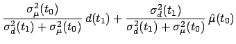
Another enlighting way of writing Eq.(30) is considering $\mu_0$ and $\mu_1$ the estimates of $\mu$ at times $t_0$ and $t_1$, respectively before and after the observation $d$ happened at time $t_1$. Indicating the estimates at different times by $\hat \mu(t)$, we can rewrite Eq.(30) as

$$\hat \mu(t_1) = \frac{\sigma_\mu^2(t_0)}{\sigma_d^2(t_1)+\sigma_\mu^2(t_0)}\, d(t_1) + \frac{\sigma_d^2(t_1)}{\sigma_d^2(t_1)+\sigma_\mu^2(t_0)}\, \hat\mu(t_0)$$

$$= \hat\mu(t_0) + \frac{\sigma_\mu^2(t_0)}{\sigma_d^2(t_1)+\sigma_\mu^2(t_0)} \, [d(t_1) - \hat\mu(t_0)]$$ (33)

$$= \hat\mu(t_0) + K(t_1) \, [d(t_1) - \hat\mu(t_0)]$$ (34)

$$\sigma_\mu^2(t_1) = \sigma_\mu^2(t_0) - K(t_1) \, \sigma_\mu^2(t_0) \,,$$ (35)

where

$$K(t_1) = \frac{\sigma_\mu^2(t_0)}{\sigma_d^2(t_1)+\sigma_\mu^2(t_0)}\,.$$ (36)

Indeed, we have given Eq.(30) the structure of a Kalman filter (Kalman 1960). The new observation `corrects' the estimate by a quantity given by the innovation (or residual) $[d(t_1) - \hat\mu(t_0)]$ times the blending factor (or gain) $K(t_1)$. For an introduction about Kalman filter and its probabilistic origin, see (Maybeck 1979 and Welch and Bishop 2002).

As Eqs. (31)-(35) show, a new experimental information reduces the uncertainty. But this is true as long the previous information and the observation are somewhat consistent. If we are, for several reasons, sceptical about the model which yields the combination rule (31)-(32), we need to remodel the problem and introduce possible systematic errors or underestimations of the quoted standard deviations, as done e.g. in (Press 1997, Dose and von der Linden 1999, D'Agostini 1999b, Fröhner 2000).