Next: General principle based priors
Up: Choice of priors -
Previous: Purely subjective assessment of
Conjugate priors
Because of computational problems,
modelling priors has been traditionally
a compromise between a realistic assessment of beliefs
and choosing a mathematical function that simplifies
the analytic calculations.
A well-known strategy is to choose a prior with a suitable form
so the posterior belongs to the same functional family as the prior.
The choice of the family depends on the likelihood. A prior
and posterior chosen in this way are said to be conjugate.
For instance, given a Gaussian likelihood and choosing a Gaussian prior,
the posterior is still Gaussian, as we have seen in
Eqs. (25), (28) and
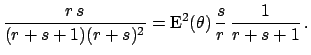
(29). This is because expressions of the form
can always be written in the form
with suitable values for  ,
,  and
and  . The Gaussian distribution
is auto-conjugate. The mathematics is simplified but, unfortunately,
only one shape is possible.
. The Gaussian distribution
is auto-conjugate. The mathematics is simplified but, unfortunately,
only one shape is possible.
An interesting case, both for flexibility and practical interest is
offered by the binomial likelihood (see Sect. 5.3).
Apart from the binomial coefficient,
 has the
shape
has the
shape
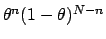 , which has the same structure as the
Beta distribution, well known to statisticians:
, which has the same structure as the
Beta distribution, well known to statisticians:
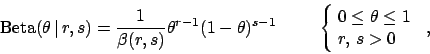 |
(94) |
where  stands for the Beta function, defined as
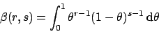 |
(95) |
which can be expressed in terms of Euler's Gamma function as
 .
Expectation
and variance of the Beta distribution are:
.
Expectation
and variance of the Beta distribution are:
If  and
and  , then the mode is unique, and it is at
 .
Depending on the value of the parameters the Beta pdf
can take a large variety of shapes.
For example, for large values of
.
Depending on the value of the parameters the Beta pdf
can take a large variety of shapes.
For example, for large values of  and
and  ,
the function is very similar to a Gaussian distribution,
while a constant function is obtained
for
,
the function is very similar to a Gaussian distribution,
while a constant function is obtained
for  . Using the Beta pdf as prior function in
inferential problems with a binomial likelihood, we have
. Using the Beta pdf as prior function in
inferential problems with a binomial likelihood, we have
The posterior distribution is still a Beta with
 and
and  , and expectation and standard
deviation can be calculated easily from Eqs. (96)
and (97).
These formulae demonstrate how the posterior estimates become
progressively independent of the prior information in the limit of
large numbers;
this happens when both
, and expectation and standard
deviation can be calculated easily from Eqs. (96)
and (97).
These formulae demonstrate how the posterior estimates become
progressively independent of the prior information in the limit of
large numbers;
this happens when both  and
and  . In this limit, we get
the same result as for a uniform prior ().
. In this limit, we get
the same result as for a uniform prior ().
Table 2:
Some useful conjugate priors.
 and
and  stand for the observed value (continuous or discrete, respectively)
and
stand for the observed value (continuous or discrete, respectively)
and  is the generic
symbol for the
parameter to infer, corresponding to
is the generic
symbol for the
parameter to infer, corresponding to  of a Gaussian, of a binomial
and
of a Gaussian, of a binomial
and  of a Poisson distribution.
| likelihood |
conjugate prior |
posterior |
 |
 |
 |
Normal
 |
Normal
 |
Normal
 [Eqs. (30)-(32)] [Eqs. (30)-(32)] |
Binomial |
Beta |
Beta |
Poisson |
Gamma |
Gamma |
Multinomial
 |
Dirichlet
 |
Dirichlet
 |
Table 2 lists some of the more useful conjugate priors.
For a more complete collection of conjugate priors,
see e.g. (Bernardo and Smith 1994, Gelman et al 1995).
Next: General principle based priors
Up: Choice of priors -
Previous: Purely subjective assessment of
Giulio D'Agostini
2003-05-13
![\begin{displaymath}
K\,\exp\left[ -\frac{(x_1-\mu)^2}{2\sigma_1^2}
-\frac{(x_2-\mu)^2}{2\sigma_2^2}\right]
\end{displaymath}](img395.png)
![\begin{displaymath}
K'\,\exp\left[ -\frac{(x'-\mu)^2}{2\sigma'^2} \right] \, ,
\end{displaymath}](img396.png)