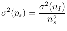
Proportion of infected individuals
in the random sample
- Binomial and hypergeometric distributions
We have already reminded and made use of the binomial
distribution, assumed well known to the reader.
A related problem in probability theory
is that of extraction without replacement,
which we introduce here for two reasons.
The first is that it is little known even by many practitioners
(we think e.g. to ourselves and to our colleagues physicists).
The second is that some care is needed
with the parameters used in literature and in
scientific/statistical libraries
of computer languages.
Let us imagine an urn containing  white and
 black balls. Let us imagine then that we are going to take out of it,
at random,
black balls. Let us imagine then that we are going to take out of it,
at random,  balls
and that we are interested in the number
balls
and that we are interested in the number  of
white balls that we shall get
(for convenience of the reader, and also for us who never
worked before with such a distribution,
we use the same idealized objects and symbols
of the R help page - obtained e.g. by `?dhyper').
The probability distribution of is known
as hypergeometric.35In short, referring to the parameters of the probability functions
of the R language (see footnote
of
white balls that we shall get
(for convenience of the reader, and also for us who never
worked before with such a distribution,
we use the same idealized objects and symbols
of the R help page - obtained e.g. by `?dhyper').
The probability distribution of is known
as hypergeometric.35In short, referring to the parameters of the probability functions
of the R language (see footnote ![[*]](crossref.png) ),
),
with expected value and variance
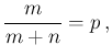
In terms of the proportion of `objects' having the characteristic
of interest (`white'), their fraction in the urn is then assumed to be
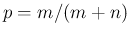 , corresponding,
in our problem, to the proportion of infectees.
Using the symbol
, corresponding,
in our problem, to the proportion of infectees.
Using the symbol  for the sample size ,
as we have done so far, and
for the sample size ,
as we have done so far, and  for the total
number of individuals in the population,
the above equations can be conveniently rewritten as
for the total
number of individuals in the population,
the above equations can be conveniently rewritten as
The expression of the expected value is identical to that
of a binomial distribution, while that of the variance differs from it by a
factor depending on the difference between the population size and
the sample size, vanishing when is equal to .
That is simply because in that case
we are going to empty the `urn' and therefore we
shall count exactly the number of `white balls'.
When, instead,
is much smaller than (and then  ), we recover the variance
of the binomial. In practice it means that the effect of
replacement, related to the chance to extract more than once
the same object, becomes negligible.
), we recover the variance
of the binomial. In practice it means that the effect of
replacement, related to the chance to extract more than once
the same object, becomes negligible.
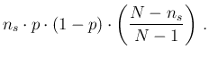
Moving to our problem, the role of the generic
variable is played by the number of infectees
in the sample, indicated by  in the previous sections.
In terms of their proportion, being
in the previous sections.
In terms of their proportion, being
 ,
we get
,
we get
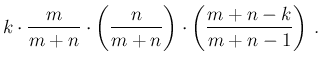
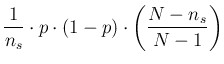
as intuitively expected. As far as the variance is concerned,
being simply
 , we get
being in all practical cases of (our) interest.
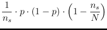
Finally, if the sample size is much smaller
than the population size, then the last
factor can be neglected and the variance
can be approximated by
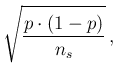
 , thus yielding
the well known standard deviation
of the fraction of successes in a binomial distribution
with trials, each with probability  . The reason is that
- it is worth repeating it -
when the sample size is much smaller than the population size,
then we can neglect the effects of no-replacement
and consider the trials as (conditionally) independent
Bernoulli processes, each with probability of success .
. The reason is that
- it is worth repeating it -
when the sample size is much smaller than the population size,
then we can neglect the effects of no-replacement
and consider the trials as (conditionally) independent
Bernoulli processes, each with probability of success .