... D'Agostini¹

Università “La Sapienza” and INFN, Roma, Italia, giulio.dagostini@roma1.infn.it

.
.
.
.
.
.
.
.
.
.
.
.
.
.
.
.
.
.
.
.
.
.
.
.
.
.
.
.
.
.

... Esposito²

Retired, alfespo@yahoo.it

.
.
.
.
.
.
.
.
.
.
.
.
.
.
.
.
.
.
.
.
.
.
.
.
.
.
.
.
.
.

... not.¹

For example we would have started choosing, in Italy, the families involved in the Auditel system [15], created with the purpose to infer the share of television programs, on the basis of which advertisers pay the TV channels. In general, in order to make sampling meaningful, the selection of individuals cannot be left to a voluntary choice that would inevitably bias the outcomes of the test campaign.

.
.
.
.
.
.
.
.
.
.
.
.
.
.
.
.
.
.
.
.
.
.
.
.
.
.
.
.
.
.

... infected ²

In fact, the test reported in Ref. [16] was claimed to be sensitive both to Immunoglobulin M (IgM), the antibody related to a current infection, and Immunoglobulin G (IgG) related to a past infection [17,18]. Obviously, the effectiveness of these kind of `serological tests' is not questioned here. In particular, two kinds of immunoglobulins will take some time to develop and they are most likely characterized by decay times. Therefore, the generic expression infected individuals (or in short infectees) has to be meant as the members of the population which hold some `property' to which the test is sensitive at the time in which it is performed.

.
.
.
.
.
.
.
.
.
.
.
.
.
.
.
.
.
.
.
.
.
.
.
.
.
.
.
.
.
.

... `probabilities'.³

If you are not used to attach a probability to numbers that might have by themselves the meaning of probability, Ref. [19] is recommended.

.
.
.
.
.
.
.
.
.
.
.
.
.
.
.
.
.
.
.
.
.
.
.
.
.
.
.
.
.
.

... intent⁴

The educational writing is an old idea that both the authors pursued in the past (see e.g. Refs. [20,21,22]), strongly believing in the necessity of making the management of uncertainty a basic tenet of scholastic (and not only) curricula.

.
.
.
.
.
.
.
.
.
.
.
.
.
.
.
.
.
.
.
.
.
.
.
.
.
.
.
.
.
.

... overlooked.⁵

This problem has been recently addressed by an article on Scientific American [23], with arguments similar to the simplistic one we are going to show in Sec. , although complemented by a rather popular visualization of the question. But we have been surprised by the lack of any reference to probability theory and to the Bayes' rule in the paper.

.
.
.
.
.
.
.
.
.
.
.
.
.
.
.
.
.
.
.
.
.
.
.
.
.
.
.
.
.
.

... response,⁶

But we hardly believe that they only provide binary information, of the kind Yes/No, and we wonder why a (although slightly) more refined scale is not reported, even discretized in a few steps, like when we rank goods and services with stars. Anyway, we shall not touch this question in the present paper, but only wanted to express here our perplexity.

.
.
.
.
.
.
.
.
.
.
.
.
.
.
.
.
.
.
.
.
.
.
.
.
.
.
.
.
.
.

... infected.⁷

This point is quite relevant when the so called false positive regards some disease with a strong social stigma (e.g. AIDS). Bad practices and negligence in dealing with test results and ignoring the population background caused genuine emotional suffering, heavy distress, up to suicide attempts [30]. The same applies in forensics, where individual freedom and justice can be badly influenced by evidence mismanagement (See Ref. [31,32] and the references there). In a less tragic context, ignoring the role of the priors can cause bad decisions to be made (see e.g. Ref. [33] for an application concerning Information Security).

.
.
.
.
.
.
.
.
.
.
.
.
.
.
.
.
.
.
.
.
.
.
.
.
.
.
.
.
.
.

... population.⁸

We remind that we are not taking into account symptoms or other reasons that would increase or decrease the probability of a particular individual to be infected. For example, the journalist of Ref. [16] tells that he had `some suspicions' he could have been infected on a plane.

.
.
.
.
.
.
.
.
.
.
.
.
.
.
.
.
.
.
.
.
.
.
.
.
.
.
.
.
.
.

....⁹

Mathematically, also negative numerator and denominator would yield a positive value of $p$, although this case makes no sense in practice, requiring $\pi_1$ smaller than $\pi_2$. Moreover, the mathematical divergence of Eq. () - of no practical relevance, as we have already commented - for $\pi_1=\pi_2$ is indeed due to the fact Eq. () and () become then $n_P = \pi_1\cdot m$ and $n_N = (1-\pi_1)\cdot m$, not depending any longer on $p$. $[$In more detail, taking $\pi_2=\pi_1-\epsilon$, we get $p=(n_P-\pi_1\cdot m+\epsilon\cdot m)/(\epsilon\cdot m)$, diverging for $\epsilon\rightarrow 0$.$]$

.
.
.
.
.
.
.
.
.
.
.
.
.
.
.
.
.
.
.
.
.
.
.
.
.
.
.
.
.
.

... rule),¹⁰

See Appendix A for details.

.
.
.
.
.
.
.
.
.
.
.
.
.
.
.
.
.
.
.
.
.
.
.
.
.
.
.
.
.
.

... `before'¹¹

This usual expression, regularly used in the literature together with the term prior, could transmit the wrong idea of time order strictly needed, leading to the absurdity that the Bayes' theorem could not be applied if one did not `declare' (to a notary?) in advance her priors. What really matters, e.g. in this specific example, is the probability that the tested person could be infected or not, taking into account all other information but the test result. (We shall comment further on the meaning and the role of the priors, in particular in Sec. .)

.
.
.
.
.
.
.
.
.
.
.
.
.
.
.
.
.
.
.
.
.
.
.
.
.
.
.
.
.
.

... caption.¹²

The reader might be surprised to see plots in which $p$ goes up to 1, but the reason is twofold: first, $p$ can be also interpreted in these plots as the purely subjective degree of belief of the expert that the tested individual is infected, independently of the test result; second, the aim of this paper is rather general and, from a physicist's perspective, $p$ could have the meaning of a detector efficiency, a branching ratio in particle decays, and whatever can be modeled by a binomial distribution.

.
.
.
.
.
.
.
.
.
.
.
.
.
.
.
.
.
.
.
.
.
.
.
.
.
.
.
.
.
.

... Factor.¹³

A more proper name could be Bayes-Turing factor, or perhaps even better Gauss-Turing factor [34], but we stick here to the conventional name.

.
.
.
.
.
.
.
.
.
.
.
.
.
.
.
.
.
.
.
.
.
.
.
.
.
.
.
.
.
.

... certainty¹⁴

This is what we assume, although we are not in the position to enter into the details.

.
.
.
.
.
.
.
.
.
.
.
.
.
.
.
.
.
.
.
.
.
.
.
.
.
.
.
.
.
.

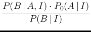
...:¹⁵

Some clarifications are provided in Appendix A. With reference to Eq. (A.8) there, Eq. () derives from

$$f(\pi_1\,\vert\,n_{P_I},n_I) \propto f(\pi_1,n_{P_I},n_I)$$

$$\propto f(n_{P_I}\,\vert\,\pi_1,n_I)\cdot f(\pi_1\,\vert\,n_I)\cdot f(n_I)$$

$$\propto f(n_{P_I}\,\vert\,\pi_1,n_I)\cdot f(\pi_1)\,,$$

in which we have used a pedantic chain rule derived from a bottom-up analysis of the second graphical model of Fig.  (the one in which $\pi_1$ is unknown) and taking into account, in the final step, that $\pi_1$ does not depend on $n_I$, which has a precise, well known value in this problem. We can note also that $f(\pi_1,n_{P_I},n_I)$ involves the continuous variable $\pi_1$ and the discrete values $n_{P_I}$ and $n_I$, being then strictly speaking neither a probability function nor a probability density function, while the meaning of each term of the chain rule is clear from the nature (continuous or discrete) of each variable (see Appendix A for details).

.
.
.
.
.
.
.
.
.
.
.
.
.
.
.
.
.
.
.
.
.
.
.
.
.
.
.
.
.
.

... unreasonable,¹⁶

Nevertheless, we shall comment in Sec.  about the practical importance of using a flat prior, because it is possible to modify the result in a second step, `reshaping' the posterior by personal, informative priors based on the best knowledge of the problem, which might be different for different experts (remember that the `prior' does not imply time order, as remarked in footnote ).

.
.
.
.
.
.
.
.
.
.
.
.
.
.
.
.
.
.
.
.
.
.
.
.
.
.
.
.
.
.

... way.¹⁷

See Sec.  for advice about the usage of mathematically convenient models.

.
.
.
.
.
.
.
.
.
.
.
.
.
.
.
.
.
.
.
.
.
.
.
.
.
.
.
.
.
.

... structure:¹⁸

Our preferred vademecum of Probability Distributions is the homonymous app [1]. More details are given in Sec. .

.
.
.
.
.
.
.
.
.
.
.
.
.
.
.
.
.
.
.
.
.
.
.
.
.
.
.
.
.
.

... test.¹⁹

To be fastidious, $s_0<1$ is not acceptable, because we do not believe a priori that a test could be perfect, and therefore $f_0(\pi_1)$ has to vanish at $\pi_1=1$. This implies that $s_0$ must be slightly above 1, for example 1.1. But in our case the observation of at least one Negative would automatically rule out $\pi_1=1$. Anyway, although this little numerical difference is irrelevant in our case, we use $s_0=1.1$ only because, since we plot priors and posteriors in Fig.  we do not like to show a prior not vanishing at 1. $[$We are admittedly a bit pedantic here for didactic purposes, but we shall be more pragmatic later (see Sec. ) and even critical about the literal use of mathematical expressions that should instead only be employed for convenience and cum grano salis (see Sec. ).$]$

.
.
.
.
.
.
.
.
.
.
.
.
.
.
.
.
.
.
.
.
.
.
.
.
.
.
.
.
.
.

... CLASS="MATH">$\pi_2=0.115$.²⁰

If, instead, we had used flat prior over the two parameters, we would get, by the Laplace' rule of succession that we shall see in a while, 0.978 and 0.124. The result is identical (within rounding) for $\pi_1$ and practically the same for $\pi_2$, because with hundreds of trials the inference is dominated by the data. (We insist in being fastidiously pedantic because of the didactic aim of this paper. For more on priors, and for the practical importance of routinely using a flat one, see Sec. .)

.
.
.
.
.
.
.
.
.
.
.
.
.
.
.
.
.
.
.
.
.
.
.
.
.
.
.
.
.
.

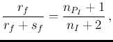
....²¹

In the case of a uniform prior, i.e. $r_0=s_0=1$, we get

$$P( \,\vert\, ) = \frac{r_f}{r_f+s_f} = \frac{n_{P_I}+1}{n_I+2}\,,$$

known as Laplace's rule of succession. In particular, for large values of $n_{P_I}$ and $n_I$, $P($Pos$\,\vert\,$Inf$)\approx n_{P_I}/n_I$: more frequently past tests applied to surely infected individuals resulted in Positive, more probably we have to expect a positive outcome of a new test of the same kind applied to an infected individual.

.
.
.
.
.
.
.
.
.
.
.
.
.
.
.
.
.
.
.
.
.
.
.
.
.
.
.
.
.
.

....²²

In principle $\pi_1$ and $\pi_2$ are not really independent, because they might depend on how the test `technology' has been optimized, and it could be easily that aiming to reach high `sensitivity' affects `specificity'. But with the information available to us we can only take them independent, each one obtained by the number of positives and negatives observed in, hopefully, well controlled samples of infected and not infected individuals.

.
.
.
.
.
.
.
.
.
.
.
.
.
.
.
.
.
.
.
.
.
.
.
.
.
.
.
.
.
.

... Carlo,²³

The rational is quite easy to understand, starting e.g. from Eq. () and remembering that $f(\pi_1,\pi_2)\,$d$\pi_1$d$\pi_2$ represents the infinitesimal probability d$P$ that $\pi_1$ and $\pi_2$ occur in the infinitesimal cell d$\pi_1$d$\pi_2$. We can discretize the plane $(\pi_1,\pi_2)$ in $N$ cells and indicate by $P_i$ the probability that a point of $\pi_1$ and $\pi_2$ falls inside it. Equation () can be approximated as

$$P( \,\vert\, ,p) \approx \sum_{i=1}^N P( \,\vert\, ,\pi_{1_i},\pi_{2_i},p) \cdot P_i$$

$$\approx \sum_{i=1}^N P( \,\vert\, ,\pi_{1_i},\pi_{2_i},p) \cdot f_i = \sum_{i=1}^N P( \,\vert\, ,\pi_{1_i},\pi_{2_i},p) \cdot \frac{n_i}{n_{tot}}\,,$$

in which we have approximated each $P_i$ by its expected relative frequency of occurrence $f_i=n_i/n_{tot}$ (Bernoulli's theorem). As one can see, we have approximated the integral by a weighted average, in which the cells in the plane that are expected to be more probable count more. In reality we do not even need to subdivide the plane into cells. We just extract at random $\pi_1$ and $\pi_2$ in the plane, according to their probability distributions, calculate $P($Inf$\,\vert\,$Pos$,\pi_{1_i},\pi_{2_i},p)$ at each point and calculate the average. When we consider a very large $n_{tot}$, then we expect that the average will not differ much from the integral.

.
.
.
.
.
.
.
.
.
.
.
.
.
.
.
.
.
.
.
.
.
.
.
.
.
.
.
.
.
.

... integral.²⁴

A similar effect happens in evaluating the contribution of systematics on measured physical quantity. If the dependence of the `influence factor' [29] is almost linear, then the `central value' is practically not affected, and only its `standard uncertainty' increases. $[$But in our case we are only interested on its `central value', that is e.g. the result of the integrals of Eqs. ()-().$]$

.
.
.
.
.
.
.
.
.
.
.
.
.
.
.
.
.
.
.
.
.
.
.
.
.
.
.
.
.
.

... independent.²⁵

The question could be a bit more sophisticated, and we have already commented in footnote on the possible dependency of $\pi_1$ and $\pi_2$. But, given the information at hand and the purpose of this paper, this is a more than reasonable assumption.

.
.
.
.
.
.
.
.
.
.
.
.
.
.
.
.
.
.
.
.
.
.
.
.
.
.
.
.
.
.

... B.1²⁶

One just needs to replace `p = 0.1' by `p = rbeta(n, 3.5, 31.5)', to be placed after n has been defined.

.
.
.
.
.
.
.
.
.
.
.
.
.
.
.
.
.
.
.
.
.
.
.
.
.
.
.
.
.
.

...tab:prob_vs_parametri.²⁷

The reason why the integral over all possible values of $p$ gives $P($Inf$\,\vert\,$Pos$)$ smaller than that obtained at a fixed value of $p$ can be understood looking at the solid red curve of Fig.  showing $P($Inf$\,\vert\,$Pos$)$ as a function of $p$ around $p=0.1$, indicated by the vertical dashed line. If $p$ has a symmetric variation around 0.1 of $\pm 0.1$ (just to make things more evident), than $P($Inf$\,\vert\,$Pos$)$ has an asymmetric variation of $^{+0.20}_{-0.47}$ around 0.476 and therefore the Monte Carlo average will be quite below 0.476 (but the Beta distribution used for $p$ is skewed on the right side and therefore there is a little compensation). For the same reason $P($NoInf$\,\vert\,$Neg$)$, practically flat in that region of $p$, is instead rather insensitive on the exact value of $p$ (unless we take unrealistic values around 0.9).

.
.
.
.
.
.
.
.
.
.
.
.
.
.
.
.
.
.
.
.
.
.
.
.
.
.
.
.
.
.

... link,²⁸

This convention is standard in the literature, although one might object - and we agree - that the opposite one would have been a better choice, a solid line better representing a deterministic link than a dashed one, but we stick to the convention.

.
.
.
.
.
.
.
.
.
.
.
.
.
.
.
.
.
.
.
.
.
.
.
.
.
.
.
.
.
.

... linearization.²⁹

See Sec. 6.4 of Ref. [2] and Sec. 8.6 of Ref. [3].

.
.
.
.
.
.
.
.
.
.
.
.
.
.
.
.
.
.
.
.
.
.
.
.
.
.
.
.
.
.

... expressions:³⁰

The first two terms of the r.h.s. of Eq. () come from Eq. (), in which the precise values $\pi_1$ and $\pi_2$ have been replaced by their expected value. The other two terms are obtained by linearization, yielding e.g. for the contribution due to $\pi_1$ (remember that $p_s$ is, so far, a precise parameter)

$$\left. \left(\frac{\partial}{\partial \pi_1} \big(\pi_1\cdot p_s\... ... n_s\big)\right)^2\right\vert _{\mbox{E}(\pi_1,\pi_2)} \! \cdot \sigma^2(\pi_1) = \big(p_s\cdot n_s\big)^2 \cdot \sigma^2(\pi_1)\,.$$

.
.
.
.
.
.
.
.
.
.
.
.
.
.
.
.
.
.
.
.
.
.
.
.
.
.
.
.
.
.

... style³¹

For this question see the ISO's GUM [29].

.
.
.
.
.
.
.
.
.
.
.
.
.
.
.
.
.
.
.
.
.
.
.
.
.
.
.
.
.
.

... rounding,³²

Using the values 0.0196 and 0.0031 of Fig. we would get 0.194.

.
.
.
.
.
.
.
.
.
.
.
.
.
.
.
.
.
.
.
.
.
.
.
.
.
.
.
.
.
.

... linearization,³³

The contribution to $\sigma^2(n_P)$ due to $\sigma(p_s)$, evaluated by linearization, is given by

$$\left. \left(\frac{\partial}{\partial p_s} \big(\pi_1\cdot p_s\cd... ..._s\big)\right)^2\right\vert _{\mbox{E}(\pi_1,\pi_2,p_s)} \! \cdot \sigma^2(p_s) = \big( (\pi_1)\cdot n_s - (\pi_2)\cdot n_s\big)^2 \cdot \sigma^2(p_s)\,.$$

.
.
.
.
.
.
.
.
.
.
.
.
.
.
.
.
.
.
.
.
.
.
.
.
.
.
.
.
.
.

... systematics.³⁴

Note that this terminology is a matter of convention and habits. From a probabilistic point of view we just apply probability theory to all quantities with respect to which we are in condition of uncertainty, considering the `fixed ones' as conditionands.

.
.
.
.
.
.
.
.
.
.
.
.
.
.
.
.
.
.
.
.
.
.
.
.
.
.
.
.
.
.

...hypergeometric.³⁵

Some care is needed with this distribution because, as it is easy to understand, different sets of parameters can be used. For example, the app already suggested [1] uses

$$X \sim (n, N, M)\,,$$

with $n$ the sample size, $N$ the population size and $M$ the number of white balls, thus leading to the following correspondence with respect to the parameters of the probability functions of the R language, to which we are going to adhere in the text

$$\longleftrightarrow$$ app R

$$n \longleftrightarrow k$$

$$N \longleftrightarrow m+n$$

$$M \longleftrightarrow m\,.$$

Expected value and variance are, using the app convention,

$$(X) = n\,\frac{M}{N}$$

$$\sigma^2(X) = n\,\frac{M}{N}\cdot\left(1 - \frac{M}{N}\right) \cdot \left(\frac{N-n}{N-1}\right)\,.$$

(In Wikipedia [4] there is a similar convention, apart from the names, being the `random variable' indicated by $k$ and the number of `white balls in the urn' by $K$.)

.
.
.
.
.
.
.
.
.
.
.
.
.
.
.
.
.
.
.
.
.
.
.
.
.
.
.
.
.
.

... Carlo.³⁶

The R code for $N=10^5$, $n_s=10^4$ and $p=0.1$ is provided in Appendix B.3.

.
.
.
.
.
.
.
.
.
.
.
.
.
.
.
.
.
.
.
.
.
.
.
.
.
.
.
.
.
.

... infectees³⁷

We remind once more that this paper is rather general, although motivated by Covid-19 related issues, and therefore we also analyze the possibility of very large $p$.

.
.
.
.
.
.
.
.
.
.
.
.
.
.
.
.
.
.
.
.
.
.
.
.
.
.
.
.
.
.

... neglected.³⁸

Indeed, in such a limit the condition () becomes

$$\begin{split} \big[\mbox{E}(\pi_1)\cdot (1-\mbox{E}(\pi_1))\c... ..._1) \cdot p^2+\sigma^2(\pi_2) \cdot (1-p)^2\big]\,, \end{split}$$

whose solution is trivial, differing from Eq. () just for the term at the denominator containing the factor $N^{-1}$.

.
.
.
.
.
.
.
.
.
.
.
.
.
.
.
.
.
.
.
.
.
.
.
.
.
.
.
.
.
.

....³⁹

This can be done evaluating $r_2$ and $s_2$ from Eqs. () and () with $\mu=0.978$ and $\sigma=0.007$.

.
.
.
.
.
.
.
.
.
.
.
.
.
.
.
.
.
.
.
.
.
.
.
.
.
.
.
.
.
.

...BUGS,⁴⁰

Introducing MCMC and related algorithms goes well beyond the purpose of this paper and we recommend Ref. [5]. Moreover, mentioning the Gibbs Sampler algorithm applied to probabilistic inference (and forecasting) it is impossible not to refer to the BUGS project [6], whose acronym stands for Bayesian inference using Gibbs Sampler, that has been a kind of revolution in Bayesian analysis, decades ago limited to simple cases because of computational problems (see also Sec. 1 of Ref.[24]). In the project web site [7] it is possible to find packages with excellent Graphical User Interface, tutorials and many examples [8].

.
.
.
.
.
.
.
.
.
.
.
.
.
.
.
.
.
.
.
.
.
.
.
.
.
.
.
.
.
.

... `object'.⁴¹

To the returned object is assigned the name `chain' in the script of Appendix B.6. In order to get information about the kind of object, just issue the command `str(chain)'.

.
.
.
.
.
.
.
.
.
.
.
.
.
.
.
.
.
.
.
.
.
.
.
.
.
.
.
.
.
.

... reasons.⁴²

Deviations from linearity are expected for $p\approx 0$ and rather small $n_s$, but, as we have checked with approximated formulae, the effect is negligible for the values of interest.

.
.
.
.
.
.
.
.
.
.
.
.
.
.
.
.
.
.
.
.
.
.
.
.
.
.
.
.
.
.

... B.8),⁴³

As alternative, one could use JAGS, of which we provide the model in Appendix B.9, leaving the R steering commands as exercise. JAGS will be instead used in Sec.  to infer $p^{(1)}$, $p^{(2)}$ and $\Delta p = p^{(2)}-p^{(1)}$.

.
.
.
.
.
.
.
.
.
.
.
.
.
.
.
.
.
.
.
.
.
.
.
.
.
.
.
.
.
.

... by⁴⁴

It might be useful to remind that, given a linear combination $Y=c_1\cdot X_1+c_2\cdot X_2$, the variance of $Y$ is given by

$$\sigma^2(Y) = c_1^2 \cdot \sigma^2(X_1) + c_2^2\cdot \sigma^2(X_2) + 2\,c_1\cdot c_2\cdot (X_1,X_2)$$

$$= c_1^2 \cdot \sigma^2(X_1) + c_2^2 \cdot \sigma^2(X_2) + 2\,c_1\cdot c_2\cdot \rho(X_1,X_2) \cdot \sigma(X_1)\cdot \sigma(X_2)\,.$$

.
.
.
.
.
.
.
.
.
.
.
.
.
.
.
.
.
.
.
.
.
.
.
.
.
.
.
.
.
.

... language.⁴⁵

The relation, ` $n_P \sim$   sum$(n_{P_I},n_{P_{NI}})$' is logically equivalent to ` $n_P <$- $n_{P_I}+n_{P_{NI}}$', but the latter instruction would not work because JAGS prohibits `observed nodes' to be defined by a deterministic assignment, as, instead, it has been done in the case of $n_{NI}$, defined as ` $n_{NI} <\!\!$- $n_s - n_I$'.

.
.
.
.
.
.
.
.
.
.
.
.
.
.
.
.
.
.
.
.
.
.
.
.
.
.
.
.
.
.

... case⁴⁶

Note that we can in principle learn something also about $\pi_1$ and $\pi_2$, because we can properly marginalize Eq. () in order to get $f(\pi_1,\pi_2\,\vert\,n_P,n_s,r_1,s_1,r_2,s_2)$. In the limit that they are very well known (condition reflected into very large $r_i$ and $s_i$) we expect that their joint probability distribution is not updated much by the new pieces of information. But, if instead they are poorly known, we get some information on them, at the expense of the quality of information we can get on the main quantity of interest, that is $p$ (although we are not going into the details, see Sec.  for a case in which $\pi_2$ is updated by the data).

.
.
.
.
.
.
.
.
.
.
.
.
.
.
.
.
.
.
.
.
.
.
.
.
.
.
.
.
.
.

... iterations.⁴⁷

Indeed the traces show that the sampling is, so to say, not optimal, and more iterations would be needed. But for our needs here and for reminding the care needed in applying this powerful tool, we prefer to show this not ideal case of sampling with a quite larger but not large enough number of iterations. (Later on, when critical, we shall increase nr up to $10^7$.)

.
.
.
.
.
.
.
.
.
.
.
.
.
.
.
.
.
.
.
.
.
.
.
.
.
.
.
.
.
.

...#tex2html_wrap_inline12370#
⁴⁸

Plot and correlation coefficient are obtained by the following R commands

chain.df <- as.data.frame( as.mcmc(chain) )
plot(chain.df, col='blue')
cor(chain.df)

.
.
.
.
.
.
.
.
.
.
.
.
.
.
.
.
.
.
.
.
.
.
.
.
.
.
.
.
.
.

... specificity.⁴⁹

In order to avoid to modify the JAGS model, we simply multiply all relevant Beta parameters by the large factor $a=10^6$, thus reducing all uncertainties by a factor thousand (see Eq. ()). This is done by adding the following command

a=1e6; r1=r1*a; s1=s1*a; r2=r2*a; s2=s2*a

.
.
.
.
.
.
.
.
.
.
.
.
.
.
.
.
.
.
.
.
.
.
.
.
.
.
.
.
.
.

....⁵⁰

We exploit the same trick of the previous item redefining the Beta parameters as follows

a=(22/7)^2;  r2=r2*a; s2=s2*a

.
.
.
.
.
.
.
.
.
.
.
.
.
.
.
.
.
.
.
.
.
.
.
.
.
.
.
.
.
.

... impossible.⁵¹

In particular, we would like to point out that this question has nothing to do with the story of the `biased estimators' of frequentists. In probabilistic inference the result is not just a single number (the famous `estimator'), but rather the distribution of the quantity of interest, of which mean and standard deviation are only some of the possible summaries, certainly the most convenient for several purposes.

.
.
.
.
.
.
.
.
.
.
.
.
.
.
.
.
.
.
.
.
.
.
.
.
.
.
.
.
.
.

... fail.⁵²

Although we cannot go through the details in this paper, it would be interesting to use `wider priors' about $\pi_1$ and $\pi_2$ in order to see how they get updated by JAGS, and then try to understand what is going on making pairwise scatter plots of the resulting $p$, $\pi_1$ and $\pi_2$.

.
.
.
.
.
.
.
.
.
.
.
.
.
.
.
.
.
.
.
.
.
.
.
.
.
.
.
.
.
.

....⁵³

It is worth pointing out the cases, occurring especially in frontier science, in which the likelihood is constant in some regions, and therefore it does not update/reshape $f_0(v)$, where `$v$' stands for the generic variable of interest (see chapter 13 of Ref. [3]). An interesting instance, in which $v$ has the role of rate of gravitational waves $r$, is discussed in Ref. [10], where the concept of relative belief updating ratio was first introduced. Another frontier physics case, applied to the Higgs boson mass $m_H$, on the basis of the experimental and theoretical information available before year 1999, is reported in Ref. [11]. The two cases are complementary because in the first one sensitivity is lost for $r\rightarrow 0$ (`likelihood open on the left side'), while in the second for $m_H\rightarrow \infty$ (`likelihood open on the right side'). (For recent developments and applications, see Ref. [12].)

.
.
.
.
.
.
.
.
.
.
.
.
.
.
.
.
.
.
.
.
.
.
.
.
.
.
.
.
.
.

... step.⁵⁴

As already remarked in footnote , `prior' does not mean that you have to declare `before' you sit down to make the inference! It just means that it is based on other pieces of information (`knowledge') on the quantity under study.

.
.
.
.
.
.
.
.
.
.
.
.
.
.
.
.
.
.
.
.
.
.
.
.
.
.
.
.
.
.

... deviation⁵⁵

See e.g. Sec. 2 of Ref. [13].

.
.
.
.
.
.
.
.
.
.
.
.
.
.
.
.
.
.
.
.
.
.
.
.
.
.
.
.
.
.

... priors.⁵⁶

The main reason of the not excellent level of agreement is due to the quite pronounced tail on the left side of the distribution. The rule could work better for other values of $n_P$, given $n_s$, but we have no interest in showing the best case and try to sell it as `typical'. We just stuck to the numeric case we have used mostly throughout the paper.

.
.
.
.
.
.
.
.
.
.
.
.
.
.
.
.
.
.
.
.
.
.
.
.
.
.
.
.
.
.

...fig:jags_inf_p_pi1_pi2.⁵⁷

The R package PearsonDS [14] also contains a random number generator, used in the script, very convenient if further Monte Carlo integrations/simulations starting from $f(p)$ are needed.

.
.
.
.
.
.
.
.
.
.
.
.
.
.
.
.
.
.
.
.
.
.
.
.
.
.
.
.
.
.

... imaginable.⁵⁸

It seems (the episode has be referred to one of us by a statistician present at the lectures) that in the 80's Dennis Lindley ended a lecture series telling something like “You see, I have shown you a wonderful, logically consistent theory. There is only a `little' problem. We are unable to do the calculations for the high dimensional problems that occur in real applications.”

.
.
.
.
.
.
.
.
.
.
.
.
.
.
.
.
.
.
.
.
.
.
.
.
.
.
.
.
.
.

....⁵⁹

Remember that all elicitations of probabilities always depend on some conditions/hypotheses/assumptions. Therefore Eq. (A.2) should be written, more properly, as

$$P(A\,\vert\,B,I) = \frac{P(B\,\vert\,A,I)\cdot P_0(A\,\vert\,I)}{P(B\,\vert\,I)}$$

with $I$ the (common!) background status of information under which all probabilities appearing in the equation are evaluated, although it is usually implicit in the equations to make them more compact, as we have done in this paper.

.
.
.
.
.
.
.
.
.
.
.
.
.
.
.
.
.
.
.
.
.
.
.
.
.
.
.
.
.
.

... connections⁶⁰

Causality is notoriously something tricky, and conditioning does not necessarily imply causation!

.
.
.
.
.
.
.
.
.
.
.
.
.
.
.
.
.
.
.
.
.
.
.
.
.
.
.
.
.
.