In Sec. ![[*]](crossref.png) we have considered
the numbers of positives and negatives that we
expect to observe, analyzing 10000 individuals,
using our initial parameters
(
we have considered
the numbers of positives and negatives that we
expect to observe, analyzing 10000 individuals,
using our initial parameters
( ,
,
 ,
,
 ) but
without taking into account the unavoidable
`statistical fluctuation'. We do it now, using the
probabilistic graphical model shown
in Fig. ,
) but
without taking into account the unavoidable
`statistical fluctuation'. We do it now, using the
probabilistic graphical model shown
in Fig. ,
Figure:
Graphical model in which the number of positives
could come from infected or not infected individuals. Arrows with
dashed lines stand for a deterministic link, being
 simply equal to the sum of
  and
and
 .
.
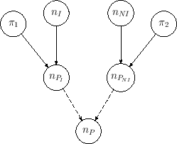 |
obtained by doubling the basic one
of Fig. , one branch
for the infectees and a second for the others. Then the numbers
of positives resulting from the two contributions are added up.
Note in Fig.
the dashed arrows from the nodes
and
to the node :
they indicate a deterministic link,28being
 .
.
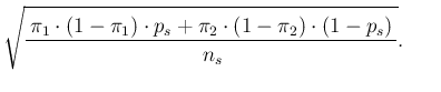
The probability distribution of  is with good approximation
Gaussian, due to the well known large numbers behavior of the
binomial distribution (and, moreover,
to the properties of the sum of `random variables').
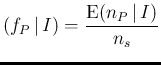
On the other hand, the expected value and the standard deviation of can been
calculated exactly, using the properties
of expected values and variances, thus getting
(summarizing for sake of space with the
symbol
is with good approximation
Gaussian, due to the well known large numbers behavior of the
binomial distribution (and, moreover,
to the properties of the sum of `random variables').
On the other hand, the expected value and the standard deviation of can been
calculated exactly, using the properties
of expected values and variances, thus getting
(summarizing for sake of space with the
symbol  , staying for all available information,
the conditions on which the
various quantities depend):
, staying for all available information,
the conditions on which the
various quantities depend):
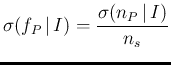
with  the sample size.
Expected value and standard deviation
of the fraction of the number of individuals
tagged as positive (
the sample size.
Expected value and standard deviation
of the fraction of the number of individuals
tagged as positive (
 ) are then
For example, making use of our reference numbers
( ,
,
 and
and
 )
we get for some
values of
)
we get for some
values of  (expected value
  standard uncertainty):
From this numbers we can get an idea about the precision
we could get on , if  and
and  were
perfectly known, although their values are rather far from
what one would ideally desire. For example, since under the hypotheses
were
perfectly known, although their values are rather far from
what one would ideally desire. For example, since under the hypotheses
 and
and  (and similar numbers are obtained
varying from
(and similar numbers are obtained
varying from  to
to  ) the expected difference of
positives is
) the expected difference of
positives is
 , it follows that,
varying by
, it follows that,
varying by  the expected number of positives would vary
by
the expected number of positives would vary
by
 . This means that, roughly speaking,
it could be possible to estimate with an uncertainty
of or better.
. This means that, roughly speaking,
it could be possible to estimate with an uncertainty
of or better.
Before taking into account the effects due to the uncertainties
of and , let us
also see how the quality of the measurement depends on the sample size.
In order to do this, we fix this time
to our arbitrary value of
and vary the sample size by about half order of
magnitude (that is
 , with
 ),
reporting in this case directly the expected
fraction of positives:
),
reporting in this case directly the expected
fraction of positives:
As we can see, if we knew perfectly and ,
already a sample of a few thousands individuals would allow us to
predict the fraction of tagged positives with a relative
uncertainty of a few percent.
However there are other effects to be taken into account:
- there is uncertainty about and ;
- the proportion of infectees in the
sample is different from that in the population
(that is, in general differs from
 );
);
- the inference from the observed numbers of positives to
, and then to , has to be done using
sound probabilistic inferential methods.