Taking into account the uncertainty on  and
and 
As we have seen in
Sec. ![[*]](crossref.png) ,
the way to take into account all possible values
of and , using the rules of probability theory,
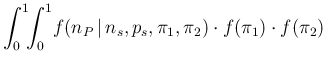
consists in evaluating the following integral
,
the way to take into account all possible values
of and , using the rules of probability theory,
consists in evaluating the following integral
Before tacking the problem of how to evaluate this integral,
a very important remark on how we are going to model
the uncertainty about and is in order.
- When we write
 , we are assuming,
trivially, the
same exact values of and for all the tests
performed on the
, we are assuming,
trivially, the
same exact values of and for all the tests
performed on the  individuals of the sample.
- If, instead, their value is uncertain, and we describe
their uncertainty by
 and
and  , again
it means that the same two numerical values influence the
results of the tests. But we just do not know
with certainty which
are these values.
, again
it means that the same two numerical values influence the
results of the tests. But we just do not know
with certainty which
are these values.
- In particular, associating to these two parameters
the pdf's and does not
mean that and fluctuate from one test to one other.
The two pdf's only describe the uncertainty on their numerical values.
- It is however reasonable to think that,
from how the `test devices' are built up, each
item could perform slightly differently than the other, but we
shall ignore
these possible test-to-test fluctuations, although
they could be taken into account just extending the model.
Going back to the practical issue of evaluating the integral,
we use again Monte Carlo methods,
employing e.g. the R script provided
in Appendix B.2, for the case of  and
and  .
The result, shown in the bottom plot of Fig. ,
.
The result, shown in the bottom plot of Fig. ,
Figure:
Probabilistic prediction of
the numbers of positives, based on a hypothetical
test on 10000 individuals, exactly 1000 of them being infected.
In the upper plot we use
 and
and
 .
In the lower plot we take into account their possible variability
(see text). The over-imposed curve shows a Gaussian with average
2013 and standard deviation 200, values obtained by the
approximated Eqs. () and ().
(The top histogram is repeated, with enlarged horizontal scale,
in Fig. .)
.
In the lower plot we take into account their possible variability
(see text). The over-imposed curve shows a Gaussian with average
2013 and standard deviation 200, values obtained by the
approximated Eqs. () and ().
(The top histogram is repeated, with enlarged horizontal scale,
in Fig. .)
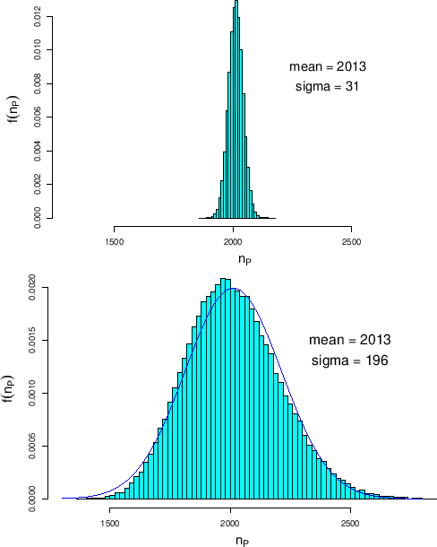 |
is quite impressive, compared to the top one, in which
the precise values
and
were used.
The mean of the distribution is unchanged,
as more or less expected (see Sec. ),
but its standard deviation, which quantifies the uncertainty of the prediction,
increases by more than a factor six.
We have then good reasons to expect
a similar effect when we will be interested in the `reverse' problem,
that is inferring the number of infectees in
the sample from the resulting number of positives.
Going into details, we see that the expected number of positives
is essentially the same of Sec.
(the reduction from 2060 to 2013 is simply due to
the new reference values for and we
are using starting from Sec. ).
But this number is now accounted by an uncertainty, which
rises to about 10% of its value, when the uncertainties
about and are also taken into account.
Subsections
 d
d