Approximated formulae

Although Monte Carlo integration is a powerful tool to solve at best non trivial problems of this kind, it is very useful to get, whenever it is possible, approximate solutions in order to have an idea, analyzing the resulting formulae, of how the result depends on the assumptions. First at all, in analogy to what we have seen in Sec. , we can be rather confident that the expected value of $n_P$ is not significantly affected, as also confirmed by the Monte Carlo results shown in Fig. . The variance, given by Eq. () is, instead, increased by terms whose approximated values can be obtained by linearization.²⁹These are the resulting approximated expressions:³⁰

$$(n_P) \approx (\pi_1)\cdot p_s\cdot n_s + (\pi_2)\cdot (1-p_s)\cdot n_s$$ (49)

$$\sigma^2(n_P) \approx (\pi_1)\cdot (1- (\pi_1)) \cdot p_s\cdot n_s + (\pi_2)\cdot (1- (\pi_2))\cdot (1-p_s)\cdot n_s$$

$$+ \,\sigma^2(\pi_1)\cdot p_s^2\cdot n_s^2 + \sigma^2(\pi_2)\cdot (1-p_s)^2\cdot n_s^2\,.$$ (50)

Applying them to the case shown in Fig.  we obtain an expected value of 2013 and a standard deviation of 200, in excellent agreement with the Monte Carlo result. In order to have an idea of the deviation from `normality' we also over-impose, to the bottom histogram of the figure, the Gaussian having average and standard deviation calculated by Eq. () and () - we remind that the top histogram has instead strong theoretical reasons to be, with very good approximation, normally distributed (a zoomed version of the same histogram is reported in Fig. ).

As a further check, let us see what happens in the case of no infected individuals in the sample, that is $p_s=0$. The Monte Carlo results are shown in Fig. ,

Figure: Same as Fig. , but in the case of no infected individual in the sample ($p_s=0$). The over-imposed Gaussian has average 1150 and standard deviation 222.

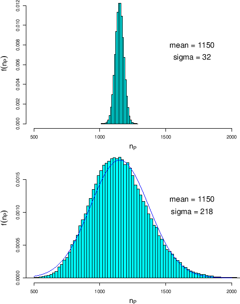We see that, as already stated qualitatively in Sec. , number of positives can occur well below the value one would compute only reasoning on rough estimates (1150 in this case). Therefore, since the formulae derived in that way were unreliable, a probabilistic treatment of the problem is needed in order to take into account the fact that fluctuations around expected values do usually occur. Also in this case the approximated results obtained by Eqs. () and () are in excellent agreement with the Monte Carlo estimates, yielding $1150 \pm 222$ (and, again, the Gaussian approximation is not too bad, at least within a couple of standard deviations from the mean value). The approximation remains good also for high values of $p_s$. For example, for the quite high value of $p_s=0.5$, the Monte Carlo integration gives $5465 \pm 116$ versus an approximated result of $5465 \pm 118$.

A natural question is how the results change not only with the proportion of infectees in the sample, but also with the size of the sample. The answer is given in Tab. , with $n_s$ varying, in steps of roughly half order of magnitude, from the ridiculous value of 100 up to 100000 (that is $\approx 10^{k/2}$, with $k=4,5,\ldots,10$).

Table: Predicted fraction of tagged positives in a sample ($f_P$) as a function of the assumed proportion of infected individuals in the sample ($p_s$), also taking into account the uncertainty on the test parameters $\pi_1$ and $\pi_2$ (numbers in squared brackets - those in round brackets are evaluated at the expected values of $\pi_1$ and $\pi_2$).

$p_s$$\rightarrow$	0.01	0.05	0.10	0.15	0.20	0.50
E$(f_P)$$\rightarrow$	0.124	0.158	0.201	0.244	0.287	0.546
$n_s$:	standard uncertainties
100	(0.032)	(0.031)	(0.031)	(0.030)	(0.029)	(0.025)
	[0.038]	[0.037]	[0.036]	[0.035]	[0.034]	[0.027]
300	(0.018)	(0.018)	(0.018)	(0.017)	(0.017)	(0.014)
	[0.028]	[0.027]	[0.026]	[0.025]	[0.024]	[0.018]
1000	(0.010)	(0.010)	(0.010)	(0.009)	(0.009)	(0.008)
	[0.024]	[0.023]	[0.022]	[0.021]	[0.020]	[0.014]
3000	(0.006)	(0.006)	(0.006)	(0.005)	(0.005)	(0.005)
	[0.022]	[0.021]	[0.020]	[0.019]	[0.018]	[0.012]
10000	(0.003)	(0.003)	(0.003)	(0.003)	(0.003)	(0.002)
	[0.022]	[0.021]	[0.020]	[0.019]	[0.018]	[0.012]
30000	(0.002)	(0.002)	(0.002)	(0.002)	(0.002)	(0.001)
	[0.021]	[0.021]	[0.020]	[0.018]	[0.017]	[0.011]
100000	(0.001)	(0.001)	(0.001)	(0.001)	(0.001)	(0.001)
	[0.021]	[0.021]	[0.019]	[0.018]	[0.017]	[0.011]

The chosen values of $p_s$ are the same of $p$ of Tab. . For an easier comparison, the fraction $f_p$ of positively tagged individual is provided. The expected value of $f_P$, depending essentially only on $p_s$, is reported in the second row of the table. Two standard uncertainties are reported for each combination of $p_s$ and $n_s$: the first, in round brackets, only takes into account the two binomial distributions (`statistical errors', in old style<sup>31</sup>physicist's jargon); the second, in square brackets takes into account also the possible variability of $\pi_1$ and $\pi_2$ (`systematic error', in the same jargon). They have all been evaluated by Monte Carlo, but the agreement with the approximated formula () has been checked.