Effect of the uncertainties on $\pi_1$ and $\pi_2$ on the probabilities of interest

The immediate question that follows is how the uncertainties concerning these two parameters change the probabilities of interest. We start reporting in Tab. 

Table: Probability of Infected and Not Infected, given the test result, as a function of the model parameters. The third and fourth rows, in boldface, are for our reference values of $\pi_1$ and $\pi_2$. The last two rows are the results `integrating over' all the possibilities of $\pi_1$ and $\pi_2$, according to Eq. () and (), with the integrals done in practice by Monte Carlo sampling.

	$p$
Probabilities
	$0.01$	$0.05$	$0.10$	$0.15$	$0.20$	$0.50$
$P($Inf$\,\vert\,$Pos$,\pi_1\!=\!0.98,\pi_2\!=\!0.12,p)$	0.0762	0.301	0.476	0.590	0.671	0.891
$P($NoInf$\,\vert\,$Neg$,\pi_1\!=\!0.98,\pi_2\!=\!0.12,p)$	0.9998	0.999	0.997	0.996	0.994	0.978
$P($Inf$\,\vert\,$Pos$,$ $\pi_1=0.978,\pi_2=0.115$$,p)$	$0.0791$	$0.309$	$0.486$	$0.600$	$0.680$	$0.895$
$P($NoInf$\,\vert\,$Neg$,$ $\pi_1=0.978,\pi_2=0.115$$,p)$	$0.9997$	$0.999$	$0.997$	$0.996$	$0.994$	$0.976$
$P($Inf$\,\vert\,$Pos$,\pi_1\!=\!0.985,\pi_2\!=\!0.115,p)$	0.0796	0.311	0.488	0.602	0.682	0.895
$P($NoInf$\,\vert\,$Neg$,\pi_1\!=\!0.985,\pi_2\!=\!0.115,p)$	0.9998	0.999	0.998	0.997	0.996	0.983
$P($Inf$\,\vert\,$Pos$,\pi_1=0.971,\pi_2=0.115,p)$	0.0786	0.308	0.484	0.598	0.679	0.894
$P($NoInf$\,\vert\,$Neg$,\pi_1=0.971,\pi_2=0.115,p)$	0.9998	0.998	0.996	0.994	0.992	0.968
$P($Inf$\,\vert\,$Pos$,\pi_1\!=\!0.978,\pi_2\!=\!0.137,p)$	0.0673	0.273	0.442	0.557	0.641	0.877
$P($NoInf$\,\vert\,$Neg$,\pi_1\!=\!0.978,\pi_2\!=\!0.137,p)$	0.9997	0.999	0.997	0.996	0.994	0.975
$P($Inf$\,\vert\,$Pos$,\pi_1=0.978,\pi_2=0.093,p)$	0.0960	0.356	0.539	0.650	0.724	0.913
$P($NoInf$\,\vert\,$Neg$,\pi_1=0.978,\pi_2=0.093,p)$	0.9998	0.999	0.997	0.996	0.994	0.976
$P($Inf$\,\vert\,$Pos$,\pi_1=0.985,\pi_2=0.093,p)$	0.0966	0.358	0.541	0.651	0.726	0.914
$P($NoInf$\,\vert\,$Neg$,\pi_1=0.985,\pi_2=0.093,p)$	0.9998	0.999	0.998	0.997	0.996	0.984
$P($Inf$\,\vert\,$Pos$,\pi_1=0.971,\pi_2=0.137,p)$	0.0668	0.272	0.441	0.556	0.639	0.876
$P($NoInf$\,\vert\,$Neg$,\pi_1=0.971,\pi_2=0.137,p)$	0.9997	0.998	0.996	0.994	0.992	0.967
$P($Inf$\,\vert\,$Pos$,\pi_1=0.985,\pi_2=0.137,p)$	0.0677	0.275	0.444	0.559	0.643	0.878
$P($NoInf$\,\vert\,$Neg$,\pi_1=0.985,\pi_2=0.137,p)$	0.9998	0.999	0.998	0.997	0.996	0.983
$P($Inf$\,\vert\,$Pos$,\pi_1=0.971,\pi_2=0.093,p)$	0.0954	0.355	0.537	0.648	0.723	0.913
$P($NoInf$\,\vert\,$Neg$,\pi_1=0.971,\pi_2=0.093,p)$	0.9997	0.998	0.996	0.994	0.992	0.969
$P($Inf$\,\vert\,$Pos$,$$p$$)$	0.0815	0.314	0.490	0.603	0.682	0.895
$P($NoInf$\,\vert\,$Neg$,$$p$$)$	0.9998	0.999	0.997	0.996	0.994	0.976

the dependence of $P($Inf$\,\vert\,$Pos$,\pi_1,\pi_2,p)$ and $P($NoInf$\,\vert\,$Neg$,\pi_1\pi_2,p)$, on which we particularly focused in the previous sections, on the three parameters. The dependence on $p$ is shown in the different columns, while the sets of $\pi_1$ and $\pi_2$ are written explicitly in the conditionands of the different probabilities. We start from the nominal values of 0.98 and 0.12 taken from Ref. [16] (first two rows of the table). Then we use the expected values calculated in the previous section (third and fourth rows, in boldface), followed by variations of $\pi_1$ and $\pi_2$ based on $\pm$ one standard deviation from their expected values.

We see that the probabilities of interest do not change significantly, the main effect being due to the assumed proportion of infectees in the population. One could argue that the dependence on $\pi_1$ and $\pi_2$ could be larger, if larger deviations of the parameters were considered. Obviously this is true, but one has to take also into account the (small) probabilities of large deviations from the mean values, especially if we allow simultaneous deviations of both parameters.

A more relevant question is, instead, how do $P($Inf$\,\vert\,$Pos$)$ and $P($NoInf$\,\vert\,$Neg) change, if we take into account all possible variations of the two parameters (weighed by their probabilities!). This is easily done, applying the result of probability theory that we have already used above. We get, for the probabilities we are mostly interested in,

$$P( \,\vert\, ,p) = \int_0^1\!\!\int_0^1\!P( \,\vert\, ,\pi_1,\pi_2,p)\cdot f(\pi_1,\pi_2)\, \pi_1 \pi_2\,.$$ (39)

$$P( \,\vert\, ,p) = \int_0^1\!\!\int_0^1\!P( \,\vert\, ,\pi_1,\pi_2,p)\cdot f(\pi_1,\pi_2)\, \pi_1 \pi_2\,,$$ (40)

where $f(\pi_1,\pi_2)$ can be factorized into $f(\pi_1)\cdot f(\pi_2)$.²²The integral can be easily done by Monte Carlo,²³whose implementation in the R language [25], both for $P($Inf$\,\vert\,$Pos$)$ and $P($NoInf$\,\vert\,$Neg$)$, is given in Appendix B.1.

We get, for our arbitrary reference value of $p=0.1$, $P($Inf$\,\vert\,$Pos$,p=0.1) = 0.49038$ and $P($NoInf$\,\vert\,$Neg$,p=0.1)=0.99727$, to be compared to 0.4858 and 0.9973, respectively, if the expected values were used. The results, shown with an exaggerated number of digits just to appreciate tiny differences, are practically the same. This result could sound counter-intuitive, especially if one thinks that $\pi_2$ has an almost 20% intrinsic standard uncertainty. The reason is due to the fact that the dependence of the probabilities of interest on $\pi_1$ and $\pi_2$ is rather linear in the region where their probability mass is concentrated, as shown in Fig. .

Figure: Dependence of $P($Inf$\,\vert\,$Pos$)$ (upper plots) and $P($NoInf$\,\vert\,$Neg$)$ (lower plots) on $\pi_1$ (left hand plots, for $\pi_2=0.115$ and $p=0.1$) and on $\pi_2$ (right hand plots, for $\pi_1=0.978$ and $p=0.1$). The parameters $\pi_1$ and $\pi_2$ are allowed to change withing a range of $\pm 3\,\sigma$'s around their expected values.

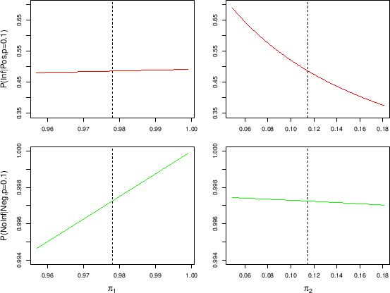This rather good linearity causes a high degree of cancellations in the integral.²⁴This explains why the only perceptible effect appears in $P($Inf$\,\vert\,$Pos$,p=0.1)$, slightly larger than the number calculated at the expected values (49.04% vs 48.58%), caused by the small non-linearity of that probability as a function of $\pi_2$, as shown in the upper, right hand plot of Fig. : symmetric variations of $\pi_2$ cause slightly asymmetric variations of $P($Inf$\,\vert\,$Pos$,p=0.1)$, thus slightly favoring higher values of that probability.