Next: Contribution of the uncertainty Up: Predicting the number of Previous: Approximated formulae Contents
![[*]](crossref.png) )
) is in order.
Its advantage,
within its limits of validity (checked in our case),
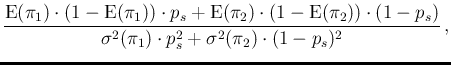
is that it allows to disentangle the contributions to the overall uncertainty.
In particular we can rewrite it as
)
) is in order.
Its advantage,
within its limits of validity (checked in our case),
is that it allows to disentangle the contributions to the overall uncertainty.
In particular we can rewrite it as
| (51) |
This quadratic combination of the contributions
can be easily extended, just dividing by ![]() ,
to the uncertainty on the fraction of positives,
thus getting
,
to the uncertainty on the fraction of positives,
thus getting
| (52) |
, the
contribution due the systematic effects alone.
For example we get, for our customary
values of ) and ():
Looking at the numbers of Tab. ,
we see that this effect starts already at ![]() .
For example, for
.
For example, for ![]() we get
we get
![]() ,
twice the standard uncertainty of 0.010 due to the binomials alone.
The sample size at which the two contributions have the
same weight in the global uncertainty is around 300
(for example, for
,
twice the standard uncertainty of 0.010 due to the binomials alone.
The sample size at which the two contributions have the
same weight in the global uncertainty is around 300
(for example, for ![]() we get
we get
![]() ).
The take-home message is, at this point,
rather clear (and well known to physicists and other scientists):
unless we are able to make our knowledge about
).
The take-home message is, at this point,
rather clear (and well known to physicists and other scientists):
unless we are able to make our knowledge about ![]() and
and ![]() more
accurate, using sample sizes much larger than 1000 is
only a waste of time.
more
accurate, using sample sizes much larger than 1000 is
only a waste of time.
However, there is still another important effect we need to consider, due to the fact that we are indeed sampling a population. This effect leads unavoidably to extra variability and therefore to a new contribution to the uncertainty in prediction (which will be somehow reflected into uncertainty in the inferential process).
Before moving to this other important effect, let us
exploit a bit more the approximated evaluation of
![]() .
For example,
solving with respect to
.
For example,
solving with respect to ![]() the condition
the condition
)-()
 |
(56) |
.
We shall go through a more complete analysis of , in which
a further contribution to the uncertainty will be also taken
into account.