Balance between statistical and systematic contributions to the uncertainty on $f_P$

The vertical dashed line in the plots of Figs. , and indicates the critical value $n_s^*$ at which the contribution to total uncertainty due to $\sigma_{\pi_2}(f_P)$ and $\sigma_{\pi_1}(f_P)$ is equal to that due to $\sigma_R(f_P)$ and $\sigma_{p_s}(f_P)$, that is for $n_s=n_s^*$ statistical and systematic contributions are equal. It follows that, due to the quadratic combination rule, the global uncertainty at that critical value of the sample size will be larger than each of them by a factor $\sqrt{2}$.

Being $n_s^*$ an important parameter in order to plan a test campaign, it is worth getting its closed, although approximated expression, obtained extending the condition () to

$$\sigma_R^2(f_P) + \sigma_{p_s}^2(f_P) = \sigma_{\pi_1}^2(f_P) + \sigma_{\pi_2}^2(f_P)\,,$$ (75)

The result, under the minimal assumption $N\gg 1$, is

$$\begin{split} n_s^*=\frac{\big[\big(\mbox{E}(\pi_1)-\mbox{E}(... ...x{E}(\pi_2)\right)^2 \cdot p \cdot (1-p)\big]/N}\,. \end{split}$$ (76)

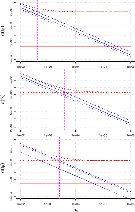
(Note how in the limit $N\gg n_s$, i.e. $N\rightarrow\infty$, the second term at the denominator of Eq. () can be neglected.³⁸) The top plot of Fig  shows the dependence of 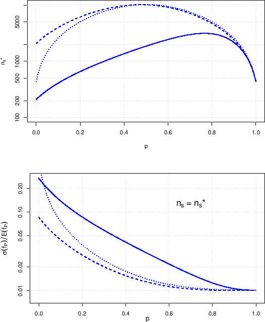$n_s^*$ on $p$,

Figure: Top plot: dependence of $n_s^*$ on $p$ for the standard values of $\sigma_{\pi_1}$ and $\sigma_{\pi_2}$ (solid line), for $\sigma_{\pi_1} = \sigma_{\pi_2} = 0.007$ (dashed line) and for specificity equal to sensitivity, i.e. E$(\pi_2)=1-$   E$(\pi_1)=0.022$ (dotted line). Bottom plot: relative uncertainty on $f_P$ at $n_s=n_s^*$ for the same cases.

for: our reference values of $\sigma(\pi_1)$ and $\sigma(\pi_2)$ (solid line - see also top plots of Figs.  and ); the improved case of $\sigma(\pi_2)=\sigma(\pi_1)=0.007$ (dashed line - see also bottom plots of Figs.  and ); the mirror-symmetric case in which E$(\pi_2)=1-$   E$(\pi_1)=0.022$ and $\sigma(\pi_2)=\sigma(\pi_1)=0.007$ (dotted line - see also Fig. ). Once we know the dependence of $n_s^*$ on $p$, since the uncertainty on $f_P$ depends on $n_s$ and $p$, we can evaluate the relative uncertainty on the predicted fraction of positives that will result from the test campaign, as a function of $p$ under the condition $n_s=n_s^*$, that is $\left.\sigma(f_P)/\mbox{E}(f_P)\right\vert _{n_s=n_s^*}$. The result is shown in the bottom plot of Fig  for the three cases of the upper plot of the same figure.

When we reduce the uncertainty about $\sigma(\pi_2)$, keeping constant its expected value, the systematic contribution to the uncertainty is reduced and then, as we have already learned from Figs. , and , it becomes meaningful to analyze larger samples. We can then predict the fraction of individuals tagged as positive with improved accuracy, i.e. $\sigma(f_P)/$E$(f_P)$ decreases. This intuitive reasoning is confirmed by the plots of Fig , moving from the solid curves to the dashed ones. Instead, improving the specificity to 0.885 to 0.978, i.e. reducing E$(\pi_2)$ from 0.115 to 0.022, keeping the same uncertainty of 0.007, leads to surprising results at low values of $p$, at least at a first sight (dashed curves $\rightarrow$ dotted curves). In fact, one would expect that from this further improvement in the quality of the test (which definitively makes a difference when testing a single individual, as discussed in Sec. ) should follow a general improvement in the prediction of the fraction of positives.

The reason of this counter-intuitive outcome is due to the combination of two effects. The first is the dependence on E$(\pi_1)$ and E$(\pi_2)$ of the statistical contributions to the uncertainty, as we can see from Eqs. () and (). The second is that, decreasing E$(\pi_2)$, the expected value of $f_P$ decreases too (less `false positives') and therefore the relative uncertainty on $f_P$, i.e. $\sigma(f_P)/$E$(f_P)$, increases. While the second effect is rather obvious and there is little to comment, we show the first one graphically, for $p=0.1$ at which the effects becomes sizable, in the three plots of Fig. :

Figure: Contributions to $\sigma(f_P)$ varying $\sigma(\pi_2)$ and E$(\pi_2)$ for $p=0.1$ (see text).

the upper plot for our reference values of $\pi_1$ and $\pi_2$, the middle one improving $\sigma(\pi_2)$ to 0.007, and the bottom one also reducing the expected value of $\pi_2$ to 0.022. But differently from Figs. , and , these plots show $\sigma(f_P)$ instead of $\sigma(f_P)/$E$(f_P)$, so that we can focus only on the contributions to the uncertainty, not `distracted' by the variation of the expected value of $f_P$. Moving from the top plot to the middle one, only the contribution due to $\pi_2$ is reduced, all the others remaining exactly the same. Then, when we increase the specificity, i.e. we reduce E$(\pi_2)$ from 0.115 to 0.022, keeping unaltered its uncertainty, its contribution to $\sigma(f_P)$ is unaffected, while the statistical contributions do change. In particular $\sigma_R(f_P)$ is strongly reduced, while $\sigma_{p_s}(f_P)$ increases a little bit. The combined effect is a decrease of the overall statistical contribution, thus lowering $n_s^*$.

Summing up, the combination of the two plots of Fig.  gives at a glance, for an assumed proportion of infectees $p$, an idea of the `optimal' relative uncertainty we can get on $f_P$ (bottom plot) and the sample size needed to achieve it (upper plot). We remind that the lowest relative uncertainty, equal to $1/\sqrt{2}$ of the value shown in the plot, is reached when the sample size $n_s$ is about one order of magnitude larger than $n_s^*$, i.e. when the random contribution to the uncertainty is absolutely negligible and any further increase of $n_s$ not justifiable. But, anyway - think about it - being $1/\sqrt{2}\approx 0.7$, is it worth increasing so much ( $\approx 10$ times) the sample size in order to reduce $\sigma(f_P)$ by only 30%?

Figure: Graphical network of Fig. , augmented by the sampling process, modeled by a hypergeometric distribution (left) or by a binomial distribution (right) with $p=N_I/(N_I+N_{NI})$.