From $P(n_{P_I}\,\vert\,n_I,\pi_1)$ to $f(\pi_1\,\vert\,n_{P_I},n_I)$: Bayes' rule applied to `numbers'

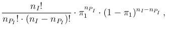
It is rather obvious to think that, repeating the same test with samples of exactly the same size, but involving different individuals, no one would be surprised to count different numbers of positives and negatives in the two samples. In fact, sticking for a while only to infectees and assuming an exact value of $\pi_1$, the number $n_{P_I}$ of positives is given by the binomial distribution,

$$f(n_{P_I}\,\vert\,n_I,\pi_1) \equiv P(n_{P_I}\,\vert\,n_I,\pi_1) = \frac{n_I!}{n_{P_I}!\cdot (n_I-n_{P_I})!}\cdot \pi_1^{n_{P_I}}\cdot (1-\pi_1)^{n_I-n_{P_I}}\,,\ \ \ \$$ (21)

that is, in short (with `$\sim$' to be read as `follows...'),

$$n_{P_I} \sim (n_I, \pi_1).$$

The probability distribution () describes how much we have to rationally believe to observe the possible values of $n_{P_I}$ (integers between 0 and $n_I$), given $n_I$ and $\pi_1$.

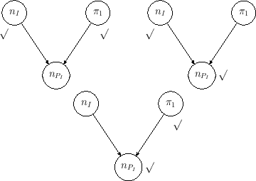
An inverse problem is to infer $\pi_1$, given $n_I$ and the observed number $n_{P_I}$ (indeed, there is also a second inverse problem, that is inferring $n_I$ from $n_{P_I}$ and $\pi_1$ - the three problems are represented graphically by the networks of Fig. ).

Figure: Graphical models of the binomial distribution (left) and its `inverse problems'. The symbol `$\surd$' indicates the `observed' nodes of the network, that is the value of the quantity associated to it is (assumed to be) certain. The other node (only one in this simple case) is `unobserved' and it is associated to a quantity whose value is uncertain.

This is the kind of Problem in the Doctrine of Chances first solved by Bayes [35], and, independently and in a more refined way, by Laplace [27] about 250 years ago. Applying the result of probability theory that nowadays goes under the name of Bayes' theorem (or Bayes' rule) that we have introduced in the previous section, we get, apart from the normalization factor $[$hereafter the same generic symbol is used for both probability functions and probability density functions (pdf), being the meaning clear from the context$]$:¹⁵

$$f(\pi_1\,\vert\,n_{P_I},n_I) \propto f(n_{P_I}\,\vert\,\pi_1,n_I) \cdot f_0(\pi_1)$$ (22)

$$\propto \pi_1^{n_{P_I}}\cdot (1-\pi_1)^{n_I-n_{P_I}} \cdot f_0(\pi_1)\,,$$ (23)

where $f_0(\pi_1)$ is the prior pdf, that describes how we believe in the possible values of $\pi_1$ `before' (see footnote and Sec. ) we get the knowledge of the experiment resulting into $n_{P_I}$ successes in $n_I$ trials. Naively one could say that all possible values of $\pi_1$ are equally possible, thus resulting in $f_0(\pi_1)=1$. But this is absolutely unreasonable,¹⁶in the case of instrumentation and procedures devised by experts in order to hopefully tag infected people as positive. Therefore the value of $\pi_1$ should be most likely in the region above $\approx 90\%$, though without sharp cut below it. Similarly, reasonable values of $\pi_2$ are expected to be in the region below $\approx 10\%$.