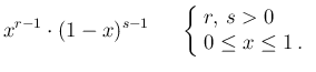
Conjugate priors

At this point, remembering Laplace's dictum that “probability is good sense reduced to a calculus”, we need to model the prior in a reasonable but mathematically convenient way.¹⁷A good compromise for this kind of problem is the Beta probability function, which we remind here, written for the generic variable

and neglecting multiplicative factors in order to focus, at this point, on its structure:¹⁸

$\displaystyle f(x\,\vert\,r,s)$

$\displaystyle \propto$

$\displaystyle x^{r-1}\cdot (1-x)^{s-1} \hspace{0.6cm}\left\{\!\begin{array}{l} r,\,s > 0 \\ 0\le x\le 1 \,. \end{array}\right.$

(24)

We see that for

a uniform distribution is recovered. An important remark is that for

the pdf vanishes at

; for

it vanishes at

. It follows that, if

and

are both above 1, we can see at a glance that the function has a single maximum. It is easy to calculate that it occurs at (`modal value')

$\displaystyle x_m$

$\displaystyle =$

$\displaystyle \frac{r-1}{r + s -2}\,.$

(25)

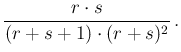
Expected value and variance ( $\sigma^2$ ) are

$\displaystyle \mu =$ E $\displaystyle (X)$	$\displaystyle =$	$\displaystyle \frac{r}{r+s}$	(26)
$\displaystyle \sigma^2 =$ Var $\displaystyle (X)$	$\displaystyle =$	$\displaystyle \frac{r\cdot s}{(r+s+1)\cdot(r+s)^2}\,.$	(27)

In the case of uniform distribution, recovered by

, we obtain the well known E

and $\sigma(X)=1/\sqrt{12}$ (and, obviously, there is no single modal value). For large

, we get $\sigma(X)\approx 1/\sqrt{8\,r}$ : as the values of

and

increases, the distribution becomes very narrow around

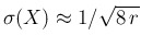
**Figure:** Examples of Beta distributions. The curves preferring small values of the generic variable , all having E are obtained with (widest to narrowest) $r=1.1,\,2,\,5,\,10$ and $s=4\,r$ ( $\sigma$ : 0.16, 0.12, 0.078, 0.056). Those preferring larger values of , all having E are obtained with (again widest to narrowest) $s=1.1,\,2,\,5$ and $r=9\,s$ ( $\sigma$ : 0.087, 0.065, 0.042).
$\begin{figure}\begin{center} \epsfig{file=esempi_beta.eps,clip=,width=\linewidth} \\ \mbox{} \vspace{-1.0cm} \mbox{} \end{center} \end{figure}$

Examples, with values of

and

to possibly model the priors we are interested in, are shown in Fig.

Using the Beta distribution for $f_0(\pi_1)$ , our inferential problem is promptly solved, since Eq. () becomes, besides a normalization factor and with parameters indicated as and in order to remind their role of prior parameters,

$\displaystyle f(\pi_1\,\vert\,n_I,n_{P_I},r_0,s_0)$	$\displaystyle \propto$	$\displaystyle \pi_1^{n_{P_I}}\cdot (1-\pi_1)^{n_I-n_{P_I}} \cdot \pi_1^{r_0-1}\,(1-\pi_1)^{s_0-1}$	(28)
	$\displaystyle \propto$	$\displaystyle \pi_1^{n_{P_I}+r_0-1}\cdot (1-\pi_1)^{(n_I-n_{P_I})+s_0-1}$	(29)

So, the posterior is still a Beta distribution, with parameters updated according to the simple rules

$\displaystyle r_f$	$\displaystyle =$	$\displaystyle r_0 + n_{P_I}$	(30)
$\displaystyle s_f$	$\displaystyle =$	$\displaystyle s_0 + (n_I-n_{P_I})\,.$	(31)

For this reason the Beta is known to be the prior conjugate of the binomial distribution. In terms of our variables,

$\displaystyle n_{P_I} \sim$ Binom $\displaystyle (n_I,\pi_1)$

$\displaystyle \Longrightarrow$

$\displaystyle \pi_1 \sim$ Beta $\displaystyle (r_0+n_{P_I},s_0+n_I-n_{P_I})\,.$

(32)

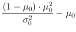
The advantage of using the Beta prior conjugate is self-evident, if we can choose values of

and

that reasonably model our prior belief about $\pi_1$ . For this reason it might be useful to invert Eq. (

) and (

), thus getting

$\displaystyle r_0$	$\displaystyle =$	$\displaystyle \frac{(1-\mu_0)\cdot \mu_0^2}{\sigma_0^2} - \mu_0$	(33)
$\displaystyle s_0$	$\displaystyle =$	$\displaystyle \frac{1-\mu_0}{\mu_0}\cdot r_0\,.$	(34)

So, for example, if we think that $\pi_1$ should be around 0.95 with a standard uncertainty of about

, we get then

and

, the latter slightly increased `by hand' to

because our rational prior has to assign zero probability to $\pi_1=1$ , that would imply the possibility of a perfect test.¹⁹The experimental data update then

and

to and . For $\pi_2$ we model a symmetric prior, with expected value 0.05 and $\sigma= 0.05$ . We just need to swap and , thus getting and , updated by the data to and . The results are shown in Fig.

**Figure:** *Priors (dashed) and posterior (solid) probability density functions of **$\pi_1$** and **$\pi_2$** .*
$\begin{figure}\begin{center} \epsfig{file=prior_posterior_pi1_pi2.eps,clip=,width=\linewidth} \\ \mbox{} \vspace{-1.0cm} \mbox{} \end{center} \end{figure}$

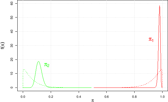Expressed in terms of expected value $\pm$ standard deviation they are

$\displaystyle \pi_1$	$\displaystyle =$	$\displaystyle 0.978 \pm 0.007$	(35)
$\displaystyle \pi_2$	$\displaystyle =$	$\displaystyle 0.115 \pm 0.022\,.$	(36)

As we can easily guess, using simply 0.98 and 0.12, as we have done in the previous sections, will give essentially the same results, in terms of expectations. Anyway, in order to be internally consistent hereafter our reference values will be $\pi_1=0.978$ and $\pi_2=0.115$ .²⁰