The probability of Infected or Not Infected,
given the result of the test,
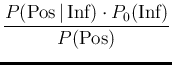
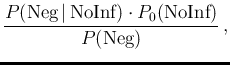
is easily calculated using a simple rule of probability theory
known as Bayes' theorem
(or Bayes' rule),10thus obtaining, for the two probabilities to which we
are interested (the other two are obtained by complement),
where  stands for the initial, or prior probability,
i.e. `before'11the information of the test result is acquired, i.e.
the degree of belief we attach to the hypothesis that a person
could be e.g. infected, based on our best knowledge
of the person (including symptoms and habits)
and of the infection.
As we have already said, if the person is chosen absolutely
at random, or we are unable to form our mind even having the person
in front of us, we can only use for
stands for the initial, or prior probability,
i.e. `before'11the information of the test result is acquired, i.e.
the degree of belief we attach to the hypothesis that a person
could be e.g. infected, based on our best knowledge
of the person (including symptoms and habits)
and of the infection.
As we have already said, if the person is chosen absolutely
at random, or we are unable to form our mind even having the person
in front of us, we can only use for
 Inf
Inf the
proportion
the
proportion  of infected individuals in the population,
or assume a value and provide probabilities
conditioned by that value, as we shall do in a while.
Therefore, hereafter the two `priors' will just be
Inf
of infected individuals in the population,
or assume a value and provide probabilities
conditioned by that value, as we shall do in a while.
Therefore, hereafter the two `priors' will just be
Inf and
NoInf
and
NoInf .
.
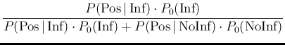
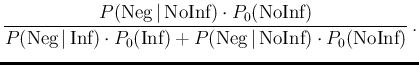
Applying another well known theorem,
since the hypotheses
Inf and
NoInf
are exhaustive and mutually exclusive, we can rewrite the above
equations as
In our model
 Pos
Pos Inf and
NegNoInf depend
on our assumptions on the parameters
Inf and
NegNoInf depend
on our assumptions on the parameters  and
and  ,
that is, including the other two probabilities of interest,
,
that is, including the other two probabilities of interest,
 Pos Pos Inf Inf |
 |
 |
(10) |
PosNoInf |
|
 |
(11) |
| NegInf |
|
 |
(12) |
| NegNoInf |
|
 |
(13) |
In the same way we can rewrite Eqs. (![[*]](crossref.png) ) and (),
adding, for completeness, also the other two probabilities of interest,
as
) and (),
adding, for completeness, also the other two probabilities of interest,
as
InfPos |
|
 |
(14) |
NoInf Neg Neg |
|
 |
(15) |
| NoInfPos |
|
 |
(16) |
| InfNeg |
|
 |
(17) |
We also remind that the denominators have the meaning of `a priori
probabilities of the test results', being
For example, taking the parameters of our numerical example
( ,
,
 and
and
 ), an individual chosen
at random is expected to be tagged as positive or negative
with probabilities
20.6% and 79.4%, respectively.
), an individual chosen
at random is expected to be tagged as positive or negative
with probabilities
20.6% and 79.4%, respectively.
Figure:
Probability that an individual chosen at random
will result Positive (red lines with positive slope) or Negative
(green lines, negative slope)
as a function of the assumed proportion of infectees
in the population.
Solid lines for
and
;
dashed for
and
 ;
dotted for
;
dotted for
 and
and
 ; dashed-dotted for
 and
and
 .
.
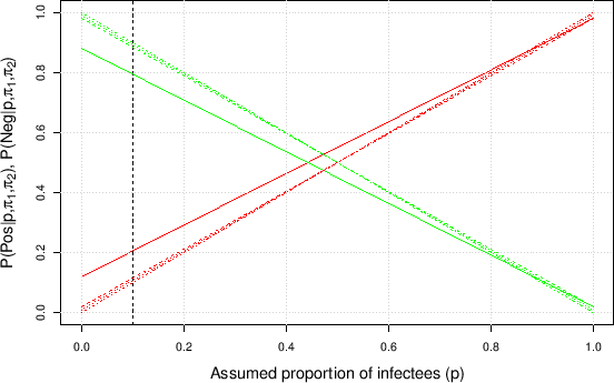 |
Figure shows these two probabilities
as a function of for some values of and .
Figure:
Probability of `Infected if tagged as Positive'
 InfPos, red line, null at
 ![$p=0\,]$](img106.png) and probability of `Not Infected if tagged as Negative'
NoInfNeg, green line, null at
and probability of `Not Infected if tagged as Negative'
NoInfNeg, green line, null at ![$p=1\,]$](img107.png) as a function of , calculated from Eqs. ()
and () for
and
(solid lines). For comparison, we have also included (dashed lines)
the case of reduced to 0.02, thus increasing the
`specificity' to 0.98. Then there are the cases
of a higher quality test
as a function of , calculated from Eqs. ()
and () for
and
(solid lines). For comparison, we have also included (dashed lines)
the case of reduced to 0.02, thus increasing the
`specificity' to 0.98. Then there are the cases
of a higher quality test
![$[\pi_1=(1-\pi_2)=0.99]$](img108.png) , shown by dotted lines
and of an extremely good test
, shown by dotted lines
and of an extremely good test
![$[\pi_1=(1-\pi_2)=0.999)]$](img109.png) shown by dotted-dashed lines.
(The probabilities to tag an individual,
chosen at random, as positive or negative,
for the same sets of parameters,
were shown in Fig. .)
shown by dotted-dashed lines.
(The probabilities to tag an individual,
chosen at random, as positive or negative,
for the same sets of parameters,
were shown in Fig. .)
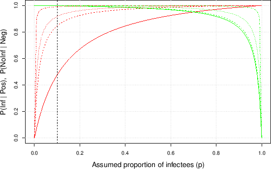 |
Figure shows,
by solid lines,
InfPos and
NoInf
and
NoInf Neg
Neg as a function of ,
having fixed and at our nominal values
0.98 and 0.12. They are identical to those
of Fig. ,
the only difference being the label of the
as a function of ,
having fixed and at our nominal values
0.98 and 0.12. They are identical to those
of Fig. ,
the only difference being the label of the  axis,
now expressed in terms of conditional probabilities.
In the same figure we have also added the results obtained
with other sets of parameters and ,
as indicated directly in the figure caption.12
axis,
now expressed in terms of conditional probabilities.
In the same figure we have also added the results obtained
with other sets of parameters and ,
as indicated directly in the figure caption.12
Analyzing the above four formulae, besides the trivial ideal condition
obtained by  and
and  , one can make
a risk analysis in order to optimize the parameters, depending
on the purpose of the test.
For example, we can rewrite Eq. () as
, one can make
a risk analysis in order to optimize the parameters, depending
on the purpose of the test.
For example, we can rewrite Eq. () as
if we want to be rather sure that a Positive is really infected, then
we need
 , unless
 .
Similarly, we can rewrite Eq. ()
as
.
Similarly, we can rewrite Eq. ()
as
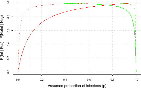
in this case, as we have learned, in order to be quite confident that the negative test implies no infection, we need
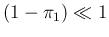 ,
that is, for realistic values of , a value of
practically equal to 1, unless is rather small,
as we can see from Fig. .
(In order to show the importance to reduce , rather
than to increase , in the case of low proportion
of infectees in the population,
we show in Fig.
the results based on some other
sets of parameters.)
,
that is, for realistic values of , a value of
practically equal to 1, unless is rather small,
as we can see from Fig. .
(In order to show the importance to reduce , rather
than to increase , in the case of low proportion
of infectees in the population,
we show in Fig.
the results based on some other
sets of parameters.)
Figure:
Same as Fig. ,
but with different parameters.
Solid lines:
and
 .
Dashed lines (the red one, describing
InfPos
overlaps perfectly
with the continuous one):
and
.
Dotted lines (the green one, describing
NoInfNeg,
almost overlaps the solid one):
and
.
.
Dashed lines (the red one, describing
InfPos
overlaps perfectly
with the continuous one):
and
.
Dotted lines (the green one, describing
NoInfNeg,
almost overlaps the solid one):
and
.
 |