Fraction of infectees in the positive sub-sample

We see therefore that, contrary to naive intuition, in spite of the apparent rather good quality of the test ( $\pi_1=0.98$), the result is quite unreliable on the individual base: a positive person has roughly 50 % chance of being really infected.⁷ But this does not mean that the test was really useless. It has indeed increased the probability of a randomly chosen individual to be infected from 10% to 48%. On the contrary, the fraction of negatives really not infected is $7920/7940 = 99.75\%$. This result is also surprising on a first sight, being the specificity $(1-\pi_2)$ only 88%, i.e. not `as good' as the sensitivity $(\pi_1)$, as high as 98%. We shall see the reason in a while. For the moment we just remark that in this second case the probability of a randomly chosen individual to be not infected has increased from 90 % to 99.75 %.

The reason of these counter-intuitive results is due to the role of the prior probability of being infected or not, based on the best knowledge of the proportion of infected individuals in the entire population.⁸The easy explanation is that, given the numbers we are playing with, the number of positives is strongly `polluted' by the large background of not infected individuals.

In order to see how the outcomes depend on $p$, let us lower its value from 10% to 1%. In this case our expectation will be of 1286 positives, out of which only 98 infected and 1188 not infected (the details are left as exercise). The fraction of positives really infected becomes now only 7.6 %. On the other hand the fraction of negatives really not infected is as high as 99.98 %. Figure

Figure: Fraction of `true positives' (red line, starting at 0 for $p=0$) and `true negatives' (green line, starting at 1 for $p=0$) in the sample, as a function of the assumed proportion $p$ of infected individuals in the population, assuming $\pi_1=P($Pos$\,\vert\,$Inf$)=0.98$ and $\pi_2= P($Pos$\,\vert\,$NoInf$) =0.12$ . The results in correspondence of $p=0.1$, arbitrarily used as reference value in the numerical example of this section, are marked by the vertical dashed line.

shows how these numbers depend on the assumed proportion of infectees in the population (and then in the sample, because of the rough reasoning we are following in this section).

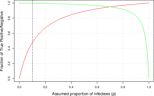This should make definitively clear that the probabilities of interest not only depend, as trivially expected, on the performances of the test, summarized here by $\pi_1$ and $\pi_2$, but also - and quite strongly! - on the assumed proportion of infectees in the population. More precisely, they depend on whether the individual shows symptoms possibly related to the searched for infection and on the probability that the same symptoms could arise from other diseases. However we are not in the condition to enter into such `details' in this paper and shall focus on random samples of the population. Therefore, up to Sec , in which we deal with the probability that a tested individual is infected or not on the basis of the test result, we shall refer to $p$ as `proportion of infectees' in the population. But everything we are going to say is valid as well if $p$ is our `prior' probability that a particular individual is infected, based on our best knowledge of the case.