More remarks on the role of priors

Having checked the agreement between the two methods, let us now focus the attention on the results themselves. Looking at the results from the smaller sample we note:

• The width of the distribution using a flat prior is wider for the small sample than that obtained with larger `statistics', as expected, with a tiny variation in the mean value: $p=0.099\pm 0.027$.
• The prior Beta$(57,38)$ causes a larger shift of the distribution towards higher values of $p$, thus yielding $p=0.204 \pm 0.015$.

It is interesting to compare these results with what we have seen in Sec.  (see Fig. ). In that case the non-flat, `informative' prior had the role of `reshaping' the posterior derived by a flat prior, making thus the result acceptable by the `expert', because the outcome was not in contrast with her prior belief. Here, instead, the result provided by a flat prior is so far from the rational belief (most likely shared by the relevant scientific community) of the expert, that the result would not be accepted acritically. Most likely the expert would mistrust the data analysis, or the data themselves. But she would perhaps also analyze critically her prior beliefs in order to understand on what they were really grounded and how solid they were. As a matter of fact, scientists are ready to modify their opinion, but with some care, and, as the famous motto says, “extraordinary claims require extraordinary evidence”.

Since scientific priors are usually strongly based on previous experimental information, the problem of `logically merging' a prior preference summarized by $\approx 0.60\pm 0.05$ and a new experimental results preferring `by itself' (that is when the result is dominated by the `likelihood' - see Sec. ), summarized as $0.098\pm 0.023$ (or $\pm 0.027$, depending on $n_s$) is similar to that of `combining apparently incompatible results.' Also in that case, nobody would acritically accept the `weighted average' of the two results which appear to be in mutual disagreement. A so called `skeptical combination' should be preferred, which would even yield a multi-modal distribution [13]. This means that in a case like those of Fig.  the expert could think that either

• she is right, with probability ${\cal P}$, and she would just stick to her prior $f_0(p)$;
• she is wrong, with probability $1-{\cal P}$, and she would switch to the posterior provided by the likelihood alone, let us indicate it with $f_{\cal L}(p)$.

Therefore the degrees of belief of $p$ will be described by $f(p) = {\cal P}\cdot f_0(p) + (1-{\cal P})\cdot f_{\cal L}(p)$. As far as we understand from our experience she would hardly believe the result obtained, `technically', plugging her prior in the formulae - and we keep repeating once more Laplace's dictum that “probability is good sense reduced to a calculus”.

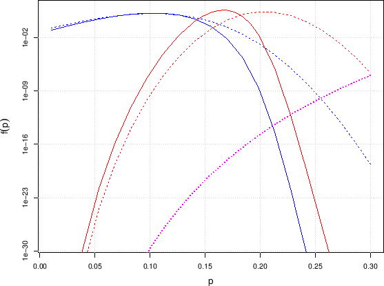
In order to make our point more clear, let us look into the details of the situation depicted in Fig.  with the help of Fig. , in which

Figure: Closer look at the effect of the prior Beta$(57,38)$ shown in Fig. .

$f(p)$ is reported in log scale, and the abscissa limited to the region of interest. The blue curves, which are dominant below $p\approx0.10$, represent the posteriors obtained by a flat prior (solid for $n_s=10000$ and $n_P=2010$; dashed for $n_s=1000$ and $n_P=201$). Then, the dotted magenta curve is the tail at small $p$ of the prior Beta$(57,58)$, which prefers values of $p$ around $\approx 0.60\pm 0.05$. Then the red curves (solid and dashed as previously) show the posterior distributions obtained by this new prior.

The shift of both distributions towards the right side is caused by the dramatic reshaping due to prior in the region between $p\approx 0.1$ and $p\approx 0.3$ in which $f_0(p\,\vert\,$Beta$(57,38))$ varies by about 25 orders of magnitudes (!). The question is then that no expert, who believes a priori that $p$ should be most likely in the region between 0.5 and 0.7 (and almost certainly not below 0.40-0.45), can have a defensible, rational belief that values of $p$ around 0.3 are $10^{\approx 25}$ times more probable than values around 0.1. More likely, once she has to give up her prior, she would consider small values of $p$ equally likely. For this reason - let us put in this way what we have said just above - she will be in the situation either to completely mistrust the new outcome, thus keeping her prior, or the other way around. The take-away message is therefore just the (trivial) reminder that mathematical models are in most practical cases just dictated by practical convenience and should not been taken literally in their extreme consequences, as Gauss promptly commented on the “defect” of his error function immediately after he had derived it [9]. Therefore our addendum to Laplace's dictum reminded above is don't get fooled by math.