Let us illustrate these ideas with a simple case on which
exact calculations can be also done:
the inference of  of a binomial distribution, based on
 successes got in
  trials.
We went through it in Sec.
trials.
We went through it in Sec. ![[*]](crossref.png) ,
but we do it solve it now with JAGS in order to provide
some details on `reshaping'.
The model is really trivial
,
but we do it solve it now with JAGS in order to provide
some details on `reshaping'.
The model is really trivial
model {
  n ~ dbin(p, N)
  p ~ dbeta(r0,s0)
}
and the full script is provided in Appendix B.12.
For  and
and  and a flat prior the JAGS result
is shown by the histogram of Fig. .
and a flat prior the JAGS result
is shown by the histogram of Fig. .
Figure:
Inference of with binomial
distributions obtained with different priors and different ways
to make use of an `informative prior' (see text).
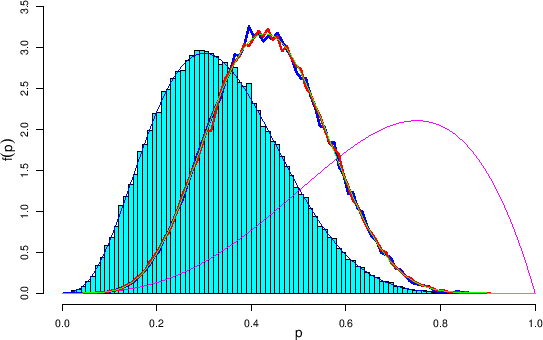 |
The blue line along the profile of the histogram
is the analytic result obtained starting from
of a Beta prior with  , that is
Beta
, that is
Beta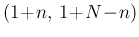 . Then the
`informative prior'
(rather vague indeed), modeled by a
Beta
. Then the
`informative prior'
(rather vague indeed), modeled by a
Beta and therefore having a mean value of
 ,
is shown by the magenta curve having the maximum
value at
,
is shown by the magenta curve having the maximum
value at
![$3/4\,=[(4-1)/(4+2-2)]$](img816.png) .
The distribution obtained reweighing the
posterior got from a flat prior
(histogram) by this new prior is shown by the blue broken curve,
while the red broken curve shows the JAGS result obtained
using the new prior (the latter curves overlap so much
that they can only be identified by color code).
Finally, the green continuous curve is the analytic
posterior obtained updating the Beta parameters, that is
Beta
.
The distribution obtained reweighing the
posterior got from a flat prior
(histogram) by this new prior is shown by the blue broken curve,
while the red broken curve shows the JAGS result obtained
using the new prior (the latter curves overlap so much
that they can only be identified by color code).
Finally, the green continuous curve is the analytic
posterior obtained updating the Beta parameters, that is
Beta .
The agreement of the three results is `perfect'
(taking into account that two of them are got by sampling).
.
The agreement of the three results is `perfect'
(taking into account that two of them are got by sampling).
The second example is our familiar case of 2010 positives
in a sample of 10000 individuals shown in detail in
Sec. and of which a different Monte Carlo
run, with
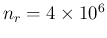 in order to get
a smoother histogram, is shown in Fig. .
in order to get
a smoother histogram, is shown in Fig. .
Figure:
Inference of the proportion
of infected in a population, having measured 2010 positives
in a sample of 10000 individuals: JAGS result based on a
flat prior (histograms) and effect of `reshaping' based
on an informative prior.
(see text).
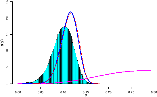 |
The new prior is indicated by the magenta curve, modeled
by a
Beta , having its mode at
 .
The reshaped posterior is indicated by the blue curve,
having mean
.
The reshaped posterior is indicated by the blue curve,
having mean  and standard deviation
  .
The result of JAGS using as prior the
Beta
is shown by the red curve, characterized by a
mean of 0.1145 and a standard deviation 0.0184
(we are using an exaggerated number of digits just for checking -
using one digit for the uncertainty both results
become `
.
The result of JAGS using as prior the
Beta
is shown by the red curve, characterized by a
mean of 0.1145 and a standard deviation 0.0184
(we are using an exaggerated number of digits just for checking -
using one digit for the uncertainty both results
become `
 ').
The degree of agreement is excellent, also taking into account that
they have intrinsic Monte Carlo fluctuations.
It is interesting to note that, besides increasing slightly the mean
values (but one could object
that “they are equal within the uncertainties”),
the main effect of the new prior is to practically rule out
values of below 0.05.
').
The degree of agreement is excellent, also taking into account that
they have intrinsic Monte Carlo fluctuations.
It is interesting to note that, besides increasing slightly the mean
values (but one could object
that “they are equal within the uncertainties”),
the main effect of the new prior is to practically rule out
values of below 0.05.